
TETA solver on the new Jean Zay Supercomputer
To be fully exploited, the massively parallel architecture of super-computers requires the use of specific software design as well as parallelization technologies and dedicated programming languages.
AxesSim had the opportunity to test its Discontinuous Galerkin (DG) TETA solver on the new Jean Zay supercomputer from CNRS, and thus demonstrate its know-how in this field.
The Discontinuous Galerkin method is well suited to the electromagnetic simulation of configurations presenting an IoT device containing a BlueTooth, Wifi or 4G / 5G antenna and placed close to the human body in order to calculate different quantities such as the SAR on the human body, the antenna radiation pattern and its electromagnetic compatibility with other devices. Indeed, the geometric constraints induced by this type of configuration are the strong point of the DG method.
Context
Context
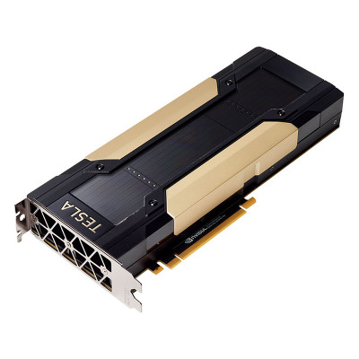
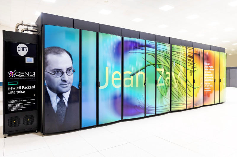
Recent scalability tests have been performed on the Jean Zay Supercomputer just launched by IDRIS. Jean Zay has 1024 Nvidia Tesla V100 32GB GPUs usable at the same time and distributed in groups of 4 on 256 nodes.
As a reminder, AxesSim (through its partnership with IRMA) benefited from computing hours as part of the “Great Challenges” initiated by IDRIS. In addition, these computing hours will also make it possible to obtain SAR results by performing simulations on the anthropomorphic mannequin formerly called Kyoto [https://www.axessim.fr/projects > HOROCH].
Once again, the very high performance of the Discontinuous Galerkin (DG) OpenCL Solver TETA, based on the generic GD-kernel CLAC – developed in partnership with IRMA Strasbourg and ONERA from Toulouse has been proved.
Scalability
Scalability performance
A preliminary study of strong scalability was carried out on a simple structured mesh, without specific physical simulation model. The purpose of this test is to assess the raw performance of the DG-OpenCL kernel of the TETA solver.
To do so, we have considered a cube of 256 hexahedra in each direction of space (for a total of about 16.8 million elements). In the case of a DG simulation in electromagnetism (EM), on hexahedra, this quantity of elements represents approximately 800 million of unknowns with the order of spatial interpolation d = 1 and respectively 2.7, 6.4 and 12.6 billion of unknowns for orders 2, 3 and 4.
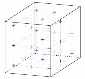
This mesh is distributed via MPI over N GPUs, for N ranging from 4 (= 22) to 256 (= 28). The MPI distribution of this mesh in the three directions was carried out in the most homogeneous way: by using a decomposition into (Nx, Ny, Nz) factors reducing the size of the interfaces :
Number of GPUs (N) Nx Ny Nz Interfaces by processus (min-max)
Number of interfaces 4 2 2 1 2-2 4 8 2 2 2 3-3 12 16 4 2 2 3-4 28 32 4 4 2 3-5 64 64 4 4 4 3-6 144 128 8 4 4 3-6 304 256 8 8 4 3-6 640
In these cases, the computation times and the MPI accelerations measured for the order d = 1 are presented here :
The ideal acceleration on N GPUs is the factor of additional GPUs compared to the reference simulation which was executed on 4 GPUs. Thus, for 256 GPUs, the theoretical acceleration is 64 (= N / 4 = 256/4).
The ideal calculation time on N GPUs is obtained by dividing the reference computation time (on 4 GPUs) by the ideal acceleration factor on N GPUs. Thus, for 8 GPUs, the ideal time is half (= 1 / (N / 4) = 4/8) of the computation time obtained on 4 GPUs.
The actual acceleration on N GPUs is obtained by calculating the ratio of the computation time on N GPUs divided by the reference time on 4 GPUs.
A quite ideal scalability up to 32 GPUs can be noticed. The increase in the number of GPUs beyond 32 still allows to observe an acceleration, but decreased by the multiplication of the number of interfaces and the reduction in the number of elements per process.
Since the TETA scalability test is performed on GPUs, the ideal acceleration is not achievable.
In fact, these interfaces in increasing number require the execution of several OpenCL kernels (extraction of EM fields, calculation of the flows and application to the time derivative) and additional MPI communications. As the number of OpenCL kernels increases and the amount of data processed by each kernel decreases, the performance becomes lower.
These performance measurements were carried out for orders 1 to 4. The MPI accelerations obtained for these different orders are presented right here :
For memory size reasons, the simulations at order 3 and 4 could only be executed from a minimum of 8 and 16 GPUs respectively. The presented accelerations are therefore calculated on the basis of the reference time obtained on 16 GPUs.
Again, we denote an acceleration up to 256 GPUs for all the interpolation orders tested. MPI scalability is better in high order, which is explained by the fact that the extraction of fields at the interfaces is less complex than the calculation of interactions in the volumes (the complexity of these two calculation steps is directly related to the interpolation order).
Application
Application cases
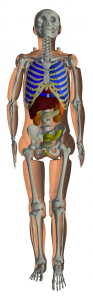
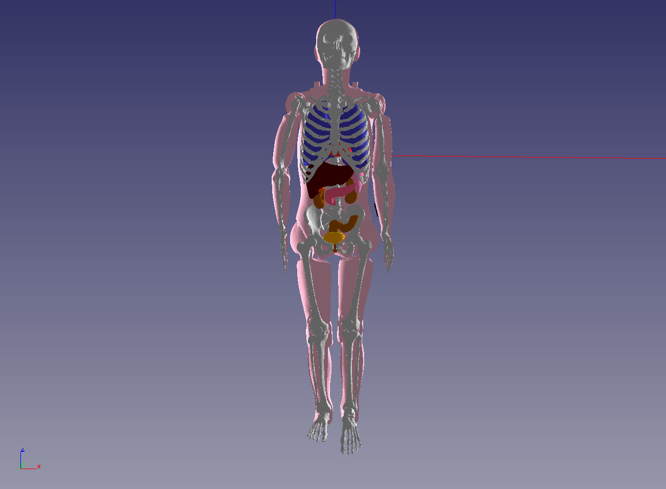
Scalability tests were also carried out in the concrete framework of the simulation on human body with a high level of geometric detail.
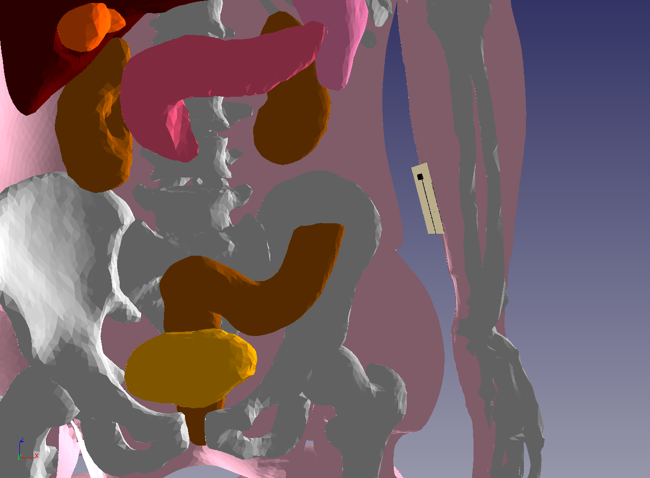
The Kyoto mannequin’s mesh has 12 organs, including the skeleton.
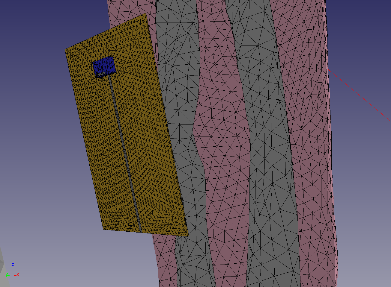
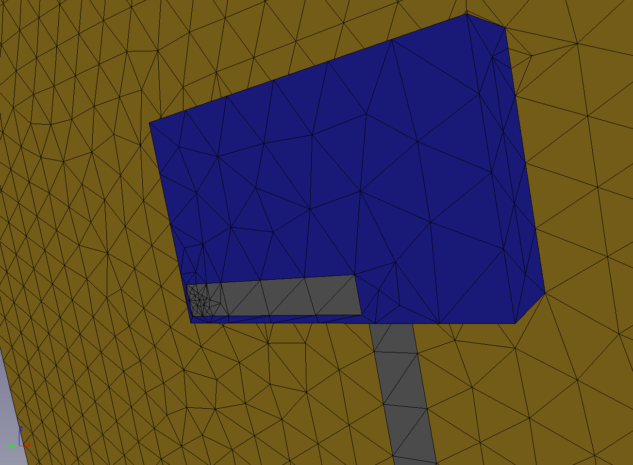
A BLE antenna of LTCC technology and radiating at 2.4 GHz was placed near the body. The maximum frequency considered for this simulation is 2.9 GHz (1 GHz band around the nominal frequency).
Scalability of the application case to the order of spatial interpolation 1
To carry out the scalability tests of the TETA solver on this simulation, it is simulated for 1000 time scheme iterations on an increasing number of GPUs. The mesh is made up of 6.7 million tetrahedra split into 26.8 million hexahedra (using the centers of the edges, faces and tetrahedron). At the maximum frequency of 2.9 GHz, the elements of the available mesh are small enough to be interpolated to order 1 in space.
Unlike the previous scalability tests, this simulation contains different physical simulation models: the injection of a signal using the antenna, dielectric volumes and an absorbing boundary condition of PML type.
For memory size reasons, our tests started with 4 GPUs and went up to 256 GPUs. The results are presented below and demonstrate significant accelerations on a larger number of GPUs :
We reach an acceleration factor of 20 on 256 GPUs compared to the time obtained on 4 GPUs. Therefore we can currently estimate that the TETA solver is approximately 80 times faster on 256 GPUs than on a single GPU.
Conclusion
The TETA solver shows an excellent scalability on massively parallel architectures encountered on modern HPCs. This tool will soon be available in the AXS-AP solution marketed by AxesSim.
The AXS-AP and AXS-E3 solutions already embed a parallel FDTD solver on CPU nodes, also offering excellent scalability performance on HPC.