8. Electromagnetic sources
Amelet HDF defines six kinds of electromagnetic sources :
- Plane wave
- Spherical wave
- Generator
- Dipole
- Antenna
- Source on mesh
They are all associated with an Amelet HDF category :
electromagneticSource/
|-- planeWave/
|-- sphericalWave/
|-- generator/
|-- antenna/
`-- sourceOnMesh/
8.1. The magnitude element
Elements in /electromagneticSource often contain a magnitude child
that is a floatingType and represents the magnitude of a source
(current generator, voltage generator, plane wave...).
magnitude has two important attributes :
delay. If the magnitude is defined in the time domain,delaywhich is a real HDF5 attribute for a time value in second represents a delay to add to the values of the floatingType.automaticMaximumValue.automaticMaximumValueis a real HDF5 attribute. If it is present, magnitude values must be scaled in order to make the maximum value magnitude equalsautomaticMaximumValue.
8.2. Plane wave
The category /electromagneticSource/planeWave contains plane wave
definitions.
A plane wave is defined by :
- A null phase point (xo, yo, zo) in meter.
- A direction of propagation in polar coordinates, in degree:
- \(\theta\), where \(\theta \in [0, \pi]\)
- \(\varphi\), where \(\varphi \in [0, 2 \pi[\)
- A polarization type :
- linear, it is defined by the angle \(\psi\) in degree
- elliptical, it is defined by \(E_{\theta}\) and \(E_{\varphi}\) that are complex electric components
- An electric field magnitude in volt per meter
The null phase point (xo, yo, zo) appears as three HDF5 real attributes xo, yo, zo.
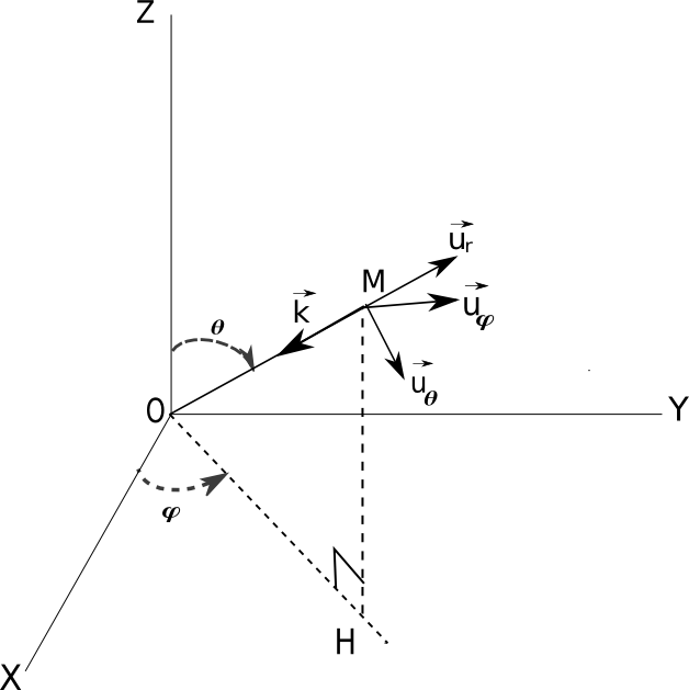
In the global cartesian coordinate system, a spherical coordinate system is defined by the two angles \((\theta, \varphi)\) which induce the three unit vectors \((\vec{u}_r, \vec{u}_{\theta}, \vec{u}_{\varphi})\).
The propagation vector is \(\vec{k}=-\frac{2\pi f}{c}.\vec{u}_r\)
and the coordinates of \((\vec{u}_r, \vec{u}_{\theta}, \vec{u}_{\varphi})\) in the global (x, y, z) coordinate system are :
\(\vec{u}_r = \begin{pmatrix} \sin\theta.\cos\varphi \\ \sin\theta.\sin\varphi \\ \cos\theta \end{pmatrix}\), \(\vec{u}_{\theta} = \begin{pmatrix} +\cos\theta.\cos\varphi \\ +\cos\theta.\sin\varphi \\ -\sin\theta \end{pmatrix}\) and \(\vec{u}_{\varphi} = \begin{pmatrix} -\sin\varphi \\ +\cos\varphi \\ 0 \end{pmatrix}\)
Wave plane definition
The electric field vector is \(\vec{E} = E_o e^{-j\vec{k}.\vec{r}}(E_{\theta}.\vec{u}_{\theta} + E_{\varphi}.\vec{u}_{\varphi})\) where \(E_o\) is the magnitude, \(E_{\theta}\) and \(E_{\varphi}\) are complex numbers (this allows to describe linear polarization and elliptical polarization)
Warning
\(E_{\theta}\) and \(E_{\varphi}\) satisfy the condition \(\|E_{\theta}.\vec{u}_{\theta} + E_{\varphi}\vec{u}_{\varphi}\|\) = 1
The magnetic field is \(\vec{H} = \frac{1}{\eta \|\vec{k}\|}.\vec{k}\wedge\vec{E}\), \(\eta\) is the wave impedance of the medium.
In Amelet HDF a plane wave is described as follows. A plane wave is a named HDF5 group.
The direction of propagation is given by :
theta, a real HDF5 attribute, it is an angle in degree and corresponds to \(\theta\)phi, a real HDF5 attribute, it is an angle in degree and corresponds to \(\varphi\)
The polarization can be “linear” or “elliptic” :
- If the polarization is linear, the HDF5 real attribute
linearPolarizationgives the value of the polarization in degree, it corresponds to \(\psi\) defined by \(E_{\theta}=\sin\psi\) and \(E_{\varphi}=\cos\psi\).
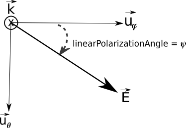
Linear polarization definition
- If the polarization is elliptical, the HDF5 complex attributes
ellipticalPolarizationETheta(corresponding to \(E_{\theta}\)) andellipticalPolarizationEPhi(corresponding to \(E_{\varphi}\)) give the definition of the polarization.
The magnitude is an Amelet HDF floatingType in volt per meter.
Example :
data.h5
`-- electromagneticSource
    `-- planeWave
        |-- $plane-wave1[@xo=0.0
        |   |            @yo=0.0
        |   |            @zo=0.0
        |   |            @theta=0.0
        |   |            @phi=0.0
        |   |            @linearPolarization=0.0]
        |    `-- magnitude[@floatingType=arraySet]
        `-- $ellipt-wave1[@xo=0.0
            |             @yo=0.0
            |             @zo=0.0
            |             @theta=0.0
            |             @phi=0.0
            |             @ellipticalPolarizationETheta=(0.0, 0.1)
            |             @ellipticalPolarizationEPhi=(0.0, 0.0)]
            `-- magnitude[@floatingType=arraySet]
8.3. Spherical wave
The category /electromagneticSource/sphericalWave contains spherical wave
definitions.
A spherical wave is defined by :
- A null phase point (xo, yo, zo) in meter.
- A power magnitude in watt.
magnitudeis afloatingType
Example :
data.h5
`-- electromagneticSource
    `-- sphericalWave
        `-- $a_spherical_wave[@xo=0.0
            |                 @yo=0.0
            |                 @zo=0.0]
            `-- magnitude[@floatingType=arraySet]
8.4. Generator
Generators are multi-pole electric devices and there are four kinds of generator in Amelet HDF :
- the voltage generator
- the current generator
- the power generator
- the power density generator
In Amelet HDF, generators are in the
/electromagneticSource/generator category.
A generator in a named HDF5 group with two floatingType children :
innerImpedancerepresenting its inner impedance in ohm.magnitudewhich is the magnitude of the signal. It is a real Amelet HDF parameter, its unit isvoltif it is a voltage generatorampereif is a current generatorwattif it is a power generatorwattPerCubicMeterif it is a power density generator
In addition it can have three optional attributes :
delay, HDF5 real attribute in second, it is time delay applied to themagnitudeinitialValue, an HDF5 real attribute, it is initial value expressed in same unit as themagnitudemaximumValue, an HDF5 real attribute, the maximum value is fixed by this attribute, a function is applied tomagnitudeto obtain those values, same unit asmagnitude.
Example
data.h5
|-- physicalModel
|   `-- multiport
|       `-- $imp1
`-- electromagneticSource
    `-- generator
        `-- $a-generator[@type=current]
            |-- innerImpedance[@floatingType=singleComplex
            |                  @physicalNature=impedance
            |                  @value=(10,0)]
            `-- magnitude[@floatingType=singleReal
                          @value=10.0]
8.5. Dipole
The category /electromagneticSource/dipole contains dipole definitions.
A dipole is a thin wire (the wire radius is wireRadius in meter),
its type can be electric
(with a length in meter) or magnetic (with a radius in meter).
Then, it is localized in the 3d space (x, y, z) and
rotated (theta, phi).
A dipole has a floatingType child loadImpedance representing
its load impedance in ohm.
Example, this Amelet HDF instance has two dipoles definition
data.h5:/electromagneticSource/dipole/elec-dipole and
data.h5:/electromagneticSource/dipole/mag-dipole
data.h5
`-- electromagneticSource
    `-- dipole
        |-- $elec-dipole[@type=electric
        |   |            @x=0.0
        |   |            @y=0.0
        |   |            @z=0.0
        |   |            @theta=0.0
        |   |            @phi=0.0
        |   |            @length=0.2
        |   |            @wireRadius=1e-4]
        |   |-- innerImpedance[@floatingType=singleComplex
        |   |                  @physicalNature=impedance
        |   |                  @value=(10,0)]
        |   `-- magnitude[@floatingType=singleReal
        |                 @delay=0.0
        |                 @value=10.0]
        `-- $mag-dipole[@type=magnetic
            |           @x=0.0
            |           @y=0.0
            |           @z=0.0
            |           @theta=0.0
            |           @phi=0.0
            |           @radius=0.2
            |           @wireRadius=1e-4]
            |-- innerImpedance[@floatingType=singleComplex
            |                  @physicalNature=impedance
            |                  @value=(10,0)]
            `-- magnitude[@floatingType=singleReal]
8.6. Antenna
Amelet HDF proposes a general description of an antenna, however some
predefined antennas are suitable. An antenna is a named group child of
/electromagneticSource/antenna category.
An antenna is defined by some electrical characteristics and radiating characteristics.
8.6.1. Electrical properties
The electrical properties are :
- The efficiency. The
efficiencyis an optional real HDF5 attribute. - The input impedance. The
inputImpedanceis an optionalfloatingTypeelement, itsphysicalNatureisimpedancevsfrequency. - The load impedance. The
loadImpedanceis an optionalfloatingTypeelement, itsphysicalNatureisimpedancevsfrequency. - The feeder impedance. The
feederImpedanceis an optionalfloatingTypeelement, itsphysicalNatureisimpedancevsfrequency. - The magnitude. The
magnitudeis an optionalfloatingTypeelement.
data.h5
`-- electromagneticSource
    `-- antenna
        `-- $antenna1[@efficiency=0.5]
            |-- inputImpedance[@floatingType=singleComplex
            |                  @physicalNature=impedance
            |                  @value=(50,0)]
            |-- loadImpedance[@floatingType=singleComplex
            |                 @physicalNature=impedance
            |                 @value=(10,0)]
            |-- feederImpedance[@floatingType=singleComplex
            |                   @physicalNature=impedance
            |                   @value=(10,0)]
            `-- magnitude[@floatingType=arraySet]
8.6.2. Radiation properties
The radiation properties of an antenna can be numerical or expressed thanks to
a predefined model. The type of an antenna is expressed in a model child
HDF5 group which has a type string attribute :
Example for a rectangular horn :
data.h5
`-- electromagneticSource/
    `-- antenna/
        `-- $antenna1[@efficiency=0.5]
            `-- model[@type=rectangularHorn
                      ...]
8.6.2.1. Numerical values
An antenna can be described by one of the following quantities :
- The gain
- it depends on theta, phi and the frequency.
gainis afloatingTypeelement child of themodelgroup .typeequalsgain
- The effective area
- It depends on theta, phi and the frequency.
effectiveAreais afloatingTypeelement child of themodelgroup.typeequalseffectiveArea
- The far field
- It depends on theta, phi and the frequency.
farFieldis afloatingTypeelement child of themodelgroup.typeequalsfarField
All these quantity are expressed in the global spherical coordinate system :
Spherical coordinate system definition
Example of an antenna defined by its gain :
data.h5
`-- electromagneticSource/
    `-- antenna/
        `-- $antenna1[@efficiency=0.5]
            `-- model[@type=gain]
                `-- gain[floatingType=arraySet]
8.6.2.2. Predefined antennas
In addition, an antenna can be one of the following predefined types :
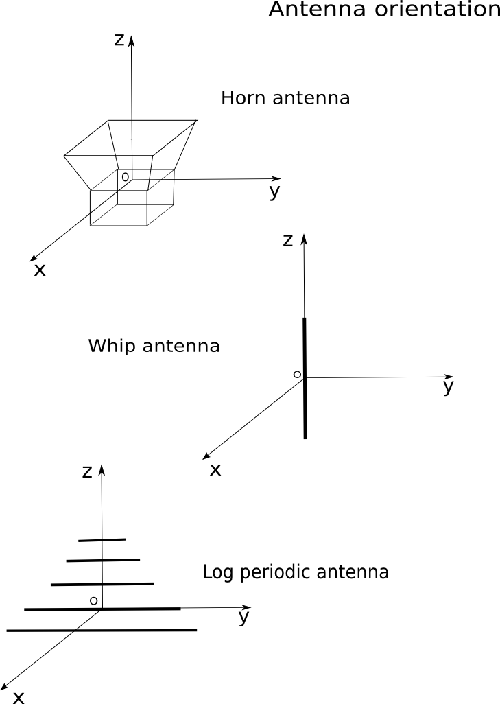
- A rectangular horn optionally with a reflector. The horn’s aperture is
in the xOy plane and radiates toward the positive-z.
apertureLargestDimension.- It is a real HDF5 attribute.
- It is the aperture’s size in the largest dimension
- A length in meter
apertureSmallestDimension- It is a real HDF5 attribute.
- It is the aperture’s size in the smallest dimension
- A length in meter
flareAngleLargestDimension- It is a real HDF5
- It is the flare angle in the largest dimension
- A angle in degree
flareAngleSmallestDimension- It is a real HDF5
- It is the flare angle in the smallest dimension
- A angle in degree
- A circular horn optionally with a reflector. The horn’s aperture is
in the xOy plane and radiates toward the positive-z .
apertureDiameter- It is a real HDF5 attribute.
- It is the aperture’s diameter
- A length in meter
flareAngle- It is a real HDF5
- It is the flare angle of the horn
- A angle in degree
- A whip antenna. The whip antenna is orthogonal to the xOy plane.
length- It is a real HDF5 attribute.
- It is the whip length
- A length in meter
radius- It is a real HDF5 attribute.
- It is the whip radius
- A length in meter
- A log periodic antenna. The array of dipole is in yOz plane and radiates
toward the positive-z.
AngularAperture- It is a real HDF5
- It is the angular aperture of the antenna
- A angle in degree
scaleFactor- It is a real HDF5
- It is the scale factor between two consecutive dipole
- without dimension
firstDipoleLength- It is a real HDF5 attribute.
- It is the length of the first dipole
- A length in meter
lastDipoleLength- It is a real HDF5 attribute.
- It is the length of the last dipole
- A length in meter
The following sketch summarizes the convention orientation for the predefined antennas :
Predefined antenna
- A generic antenna is defined by
- An
angularAperturereal HDF5 attribute which corresponds to the angular aperture of the antenna. - A
patternHDF5 string attribute, its possible values are :omnidirectionalgaussiancosecante
- An
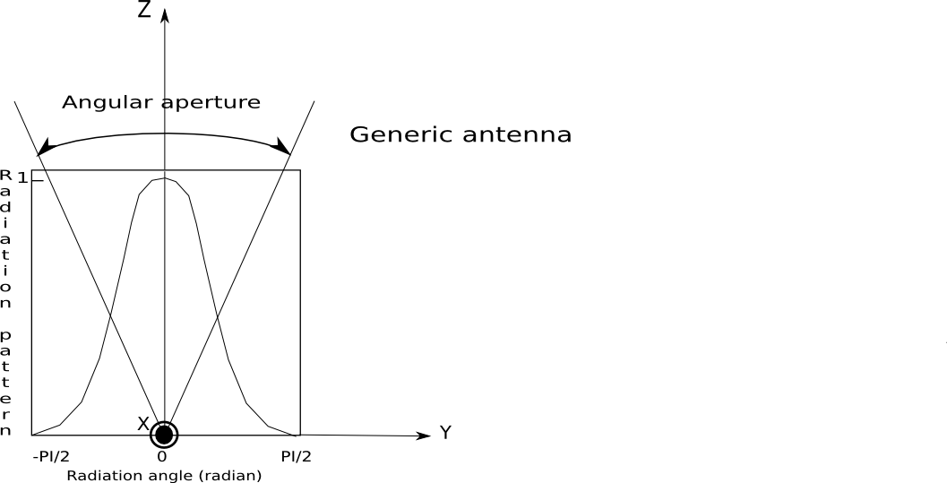
Generic antenna
Note
A generic antenna has an axis-z revolution symmetry
We have seen that a horn antenna could have a reflector. Only parabolic reflector is defined in Amelet HDF.
A parabolic reflector is a parabolicReflector HDF5 group contained in
the model group if type is rectangularHorn or circularHorn.
Parabolic reflector has three mandatory attributes
type.typeis a string HDF5 attribute and is eithercircularorrectangularIf
typeiscircular, thediameterattribute is used to give the diameter of the reflector. It is a real HDF5 attribute in meterIf
typeisrectangular, thelengthandwidthattributes are used to give the length and the width ofthe reflector. It is a real HDF5 attribute in meter
focalLength. It is a real HDF5 attribute in meter, it represents the focal length of the reflector.aspectAngle
Example for a rectangular horn with a circular reflector :
data.h5
`-- electromagneticSource/
    `-- antenna/
        `-- $antenna1[@efficiency=0.5]
            `-- model[@type=rectangularHorn
                |      ...]
                `-- parabolicReflector[@focalLength=0.2
                                       @aspectAngle=1.
                                       @type=circular
                                       @diameter=1.0]
8.6.3. Definition by example
A rectangular horn antenna with a circular reflector :
data.h5
`-- electromagneticSource
    `-- antenna
        `-- $rectHorn[@efficiency=0.5]
            |-- inputImpedance[@floatingType=singleComplex
            |                  @physicalNature=impedance
            |                  @value=(50,0)]
            |-- loadImpedance[@floatingType=singleComplex
            |                 @physicalNature=impedance
            |                 @value=(10,0)]
            |-- feederImpedance[@floatingType=singleComplex
            |                   @physicalNature=impedance
            |                   @value=(10,0)]
            |-- magnitude[@floatingType=arraySet
            |             @delay=1e-6]                 # measure : time
            |           ...
            `-- model[@type=rectangularHorn
                |     @apertureLargestDimension=0.2    # measure : length
                |     @apertureSmallestDimension=0.1   # measure : length
                |     @flareAngleLargestDimension=0.2  # measure : angle
                |     @flareAngleSmallestDimension=0.1 # measure : angle
                `-- parabolicReflector[@focalLength=0.2
                                       @aspectAngle=1.
                                       @type=circular
                                       @diameter=1.0]
A rectangular horn antenna with a rectangular reflector :
data.h5
`-- electromagneticSource
    `-- antenna
        `-- $rectHorn[@efficiency=0.5]
            |-- inputImpedance[@floatingType=singleComplex
            |                  @physicalNature=impedance
            |                  @value=(50,0)]
            |-- loadImpedance[@floatingType=singleComplex
            |                 @physicalNature=impedance
            |                 @value=(10,0)]
            |-- feederImpedance[@floatingType=singleComplex
            |                   @physicalNature=impedance
            |                   @value=(10,0)]
            |-- magnitude[@floatingType=arraySet
            |             @delay=1e-6]                  # measure : time
            |           ...
            `-- model[@type=rectangularHorn
                |     @apertureLargestDimension=0.2     # measure : length
                |     @apertureSmallestDimension=0.1    # measure : length
                |     @flareAngleLargestDimension=0.2   # measure : angle
                |     @flareAngleSmallestDimension=0.1  # measure : angle
                `-- parabolicReflector[@focalLength=0.2 # measure : length
                                       @aspectAngle=1.
                                       @type=rectangular
                                       @length=1.0      # measure : length
                                       @with=1.0]       # measure : length
A circular horn antenna :
data.h5
`-- electromagneticSource
    `-- antenna
        `-- $circHorn[@efficiency=0.5]
            |-- inputImpedance[@floatingType=singleComplex
            |                  @physicalNature=impedance
            |                  @value=(50,0)]
            |-- loadImpedance[@floatingType=singleComplex
            |                 @physicalNature=impedance
            |                 @value=(10,0)]
            |-- feederImpedance[@floatingType=singleComplex
            |                   @physicalNature=impedance
            |                   @value=(10,0)]
            |-- magnitude[@floatingType=arraySet
            |             @delay=1e-6]                 # measure : time
            |           ...
            `-- model[@type=circularHorn
                      @apertureDiameter=0.2            # measure : length
                      @flareAngle=0.2                  # measure : angle
                     ]
A log periodic antenna :
data.h5
`-- electromagneticSource
    `-- antenna
        `-- $logperiodic[@efficiency=0.5]
            |-- inputImpedance[@floatingType=singleComplex
            |                  @physicalNature=impedance
            |                  @value=(50,0)]
            |-- loadImpedance[@floatingType=singleComplex
            |                 @physicalNature=impedance
            |                 @value=(10,0)]
            |-- feederImpedance[@floatingType=singleComplex
            |                   @physicalNature=impedance
            |                   @value=(10,0)]
            |-- magnitude[@floatingType=arraySet
            |             @delay=1e-6]
            |           ...
            `-- model[@type=logPeriodic
                      @apertureAngle=0.2
                      @scaleFactor=0.1
                      @firstDipoleLength=0.1
                      @lastDipoleLength=0.7]
A whip antenna :
data.h5
`-- electromagneticSource
    `-- antenna
        `-- $whip[@efficiency=0.5]
            |-- inputImpedance[@floatingType=singleComplex
            |                  @physicalNature=impedance
            |                  @value=(50,0)]
            |-- loadImpedance[@floatingType=singleComplex
            |                 @physicalNature=impedance
            |                 @value=(10,0)]
            |-- feederImpedance[@floatingType=singleComplex
            |                   @physicalNature=impedance
            |                   @value=(10,0)]
            |-- magnitude[@floatingType=arraySet
            |             @delay=1e-6]                 # measure : time
            |           ...
            `-- model[@type=whip
                      @length=0.2                      # measure : length
                      @radius=0.1]                     # measure : angle
A generic antenna :
data.h5
`-- electromagneticSource
    `-- antenna
        `-- $generic[@efficiency=0.5]
            |-- inputImpedance[@floatingType=singleComplex
            |                  @physicalNature=impedance
            |                  @value=(50,0)]
            |-- loadImpedance[@floatingType=singleComplex
            |                 @physicalNature=impedance
            |                 @value=(10,0)]
            |-- feederImpedance[@floatingType=singleComplex
            |                   @physicalNature=impedance
            |                   @value=(10,0)]
            |-- magnitude[@floatingType=arraySet
            |             @delay=1e-6]
            `-- model[@type=generic
                      @angularAperture=0.1
                      @pattern=gaussian]               # omnidirectional
                                                       # gaussian
                                                       # cosecante
An antenna defined by a gain :
data.h5
`-- electromagneticSource
    `-- antenna
        `-- $by-gain[@efficiency=0.5]
            |-- inputImpedance[@floatingType=singleComplex
            |                  @physicalNature=impedance
            |                  @value=(50,0)]
            |-- loadImpedance[@floatingType=singleComplex
            |                 @physicalNature=impedance
            |                 @value=(10,0)]
            |-- feederImpedance[@floatingType=singleComplex
            |                   @physicalNature=impedance
            |                   @value=(10,0)]
            |-- magnitude[@floatingType=arraySet
            |             @delay=1e-6                  # measure : time
            |             @initialValue=0]
            `-- model[@type=gain]
                `-- gain[floatingType=arraySet]
An antenna defined by the effective area :
data.h5
`-- electromagneticSource
    `-- antenna
        `-- $by-area[@efficiency=0.5]
            |-- inputImpedance[@floatingType=singleComplex
            |                  @physicalNature=impedance
            |                  @value=(50,0)]
            |-- loadImpedance[@floatingType=singleComplex
            |                 @physicalNature=impedance
            |                 @value=(10,0)]
            |-- feederImpedance[@floatingType=singleComplex
            |                   @physicalNature=impedance
            |                   @value=(10,0)]
            |-- magnitude[@floatingType=arraySet
            |             @delay=1e-6]                 # measure : time
            `-- model[@type=effectiveArea]
                `-- effectiveArea[@floatingType=arraySet]
An antenna defined by the far field :
data.h5
`-- electromagneticSource
    `-- antenna
        -- $by-field[@efficiency=0.5]
            |-- inputImpedance[@floatingType=singleComplex
            |                  @physicalNature=impedance
            |                  @value=(50,0)]
            |-- loadImpedance[@floatingType=singleComplex
            |                 @physicalNature=impedance
            |                 @value=(10,0)]
            |-- feederImpedance[@floatingType=singleComplex
            |                   @physicalNature=impedance
            |                   @value=(10,0)]
            |-- magnitude[@floatingType=arraySet
            |             @delay=1e-6]                 # measure : time
            `-- model[@type=farField]
                `-- farField[@floatingType=arraySet]
An antenna defined by an exchange surface :
data.h5
|-- mesh
|   `-- $gmesh1
|       `-- $mesh1
|-- exchangeSurface
|   `-- $exchange-surface
`-- electromagneticSource
    `-- antenna
        -- $by-field[@efficiency=0.5]
            |-- inputImpedance[@floatingType=singleComplex
            |                  @physicalNature=impedance
            |                  @value=(50,0)]
            |-- loadImpedance[@floatingType=singleComplex
            |                 @physicalNature=impedance
            |                 @value=(10,0)]
            |-- feederImpedance[@floatingType=singleComplex
            |                   @physicalNature=impedance
            |                   @value=(10,0)]
            |-- magnitude[@floatingType=arraySet
            |             @delay=1e-6]                 # measure : time
            `-- model[@type=exchangeSurface
                      @exchangeSurface=/exchangeSurface/$exchange-surface]
8.7. Source on mesh
8.7.1. Data on mesh
An electromagnetic source can be set by using numerical data on mesh (see Numerical data on mesh for details).
data.h5
|-- mesh
|   `-- $gmesh1
|       `-- $mesh1
|           `-- group
|               `-- $group1
`-- electromagneticSource
    `-- sourceOnMesh
        `-- $by-data-on-mesh[@type=arraySet
            |                @label=Electric field]
            |-- data[@label=electric field
            |        @physicalNature=electricField
            |        @unit=voltPerMeter]
            `-- ds/
                |-- dim1[@label=component x y z
                |        @physicalNature=component]
                |-- dim2[@label=mesh elements
                |        @physicalNature=meshEntity]
                `-- dim3[@label=the time
                         @physicalNature=time
                         @unit=second]
with /floatingType/$dataOne/ds/dim2 :
| /mesh/$gmesh1/$mesh1/group/$group1 |
In the preceding example, data on mesh named
data.h5:/electromagneticSource/sourceOnMesh/$by-data-on-mesh is used
as an electromagneticSource of type sourceOnMesh. It relies on the
mesh group data.h5:/mesh/$gmesh1/$mesh1/group/$group1.
8.7.2. Exchange surface
data.h5
|-- exchangeSurface
|   `-- $exchange-surface
`-- electromagneticSource
    `-- sourceOnMesh
        `-- $by-ex-surf[@type=exchangeSurface
                        @exchangeSurface=/exchangeSurface/$exchange-surface]
8.7.3. Dipole cloud
A dipole cloud source is a source characterized by an optional electric dipole cloud and an optional magnetic dipole cloud. This kind of source is often generated by a signal processing step to obtain an equivalent source which radiates as a given antenna.
A dipole cloud is an arraySet where data are scalar values (electric current
or magnetic current) and dimensions are:
- A mesh support: the edge set which gives the position and the orientation of the dipoles. The edge’s length is important for the dipole cloud source model
- A dimension which gives the interval and the definition domain of the source: in time or frequency domain
The electric dipole cloud and the magnetic dipole cloud are named
respectively electricDipoleCloud and magneticDipoleCloud.
An example of dipole cloud source is given hereafter:
data.h5
|-- mesh
|   `-- $gmesh1
|       `-- $mesh1
|           `-- group
|               |-- $electric-dipole-group
|               `-- $magnetic-dipole-group
`-- electromagneticSource
    `-- sourceOnMesh
        `-- $by-dipole-cloud[@type=dipoleCloud
            |                @label=Patch antenna equivalent dipole cloud source]
            |-- electricDipoleCloud[@floatingType=arraySet
            |   |                   @label=Electric dipole cloud]
            |   |-- data[@label=Electric dipole values
            |   |        @physicalNature=electricCurrent
            |   |        @unit=ampere]
            |   `-- ds
            |       |-- dim1[@label=mesh elements
            |       |        @physicalNature=meshEntity]
            |       `-- dim2[@label=the time
            |                @physicalNature=time
            |                @unit=second]
            |                @label=Patch antenna equivalent dipole cloud source]
            `-- magneticDipoleCloud[@floatingType=arraySet
                |                   @label=Magnetic dipole cloud]
                |-- data[@label=Magnetic dipole values
                |        @physicalNature=magneticCurrent
                |        @unit=volt]
                `-- ds
                    |-- dim1[@label=mesh elements
                    |        @physicalNature=meshEntity]
                    `-- dim2[@label=the time
                             @physicalNature=time
                             @unit=second]