9. Physical models
The material models category contains models used in electromagnetic simulation like :
- Dielectric material
- Debye material
- Lorentz material
- Multi layer material for composite elements
- Electrical models
- sub-cellular models
- Slot model
- Special interfaces
Sub-categories are documented in the next sections.
9.1. Frequency range of validity
For large spectrum simulation, one material model could not be valid for the entire frequency range, so several models have to be used.
Material model have two optional real parameters (two HDF5 real attributes) :
frequency_validity_minis the minimum frequency of validity in Hertzfrequency_validity_maxis the maximum frequency of validity in Hertz
For example
data.h5
`-- physicalModel/
    `-- volume
        `-- $water[@frequency_validity_min=1e3
                   @frequency_validity_max=1e9]
9.2. Predefined model
Amelet HDF predefines some remarkable materials :
/physicalModel/perfectElectricConductor, it is the perfect electric condutor material./physicalModel/perfectMagneticConductor, it is the perfect magnetic conductor material./physicalModel/vacuum, it represents the EM vacuum.
Note
Predefined material nodes must exist in the Amelet-HDF instance
data.h5
`-- physicalModel/
    |-- perfectElectricConductor
    |-- perfectMagneticConductor
    |-- vacuum
    `-- volume
        `-- $water[@frequency_validity_min=1e3
                   @frequency_validity_max=1e9]
9.3. Volume
A volume material is a material defined by
- a relative permittivity (dimensionless)
- a relative permeability (dimensionless)
- a electric conductivity (in siemens / meter)
- a magnetic conductivity (in farad / meter), (this conductivity is used in perfectly matched layers (PML) models for instance).
- a volumetric mass density (in kilogram / cubic meter)
Such a material is a named HDF5 group child of /physicalModel/volume.
The name of the group is the name of the material.
For a material called $diel1 the tree schema looks like
data.h5
`-- physicalModel/
    `-- volume
        `-- $diel1[@volumetricMassDensity=1000.]
            |-- relativePermittivity
            |-- relativePermeability
            |-- electricConductivity
            `-- magneticConductivity
The next sections explain how the four components are defined.
9.3.1. Relative permittivity
The relative permittivity is a named HDF5 group, its name is
relativePermittivity and can be expressed in different manners :
- By a complex value
- By an array of complex values
- By a general rational function
- By a Debye model
- By a Lorentz model
9.3.1.1. Complex value
If the relative permittivity is defined by a complex number,
relativePermittivity group is a floatingType singleComplex.
relativePermittivity has no children.
Example :
data.h5
`-- physicalModel/
    `-- volume
        `-- $water
            `-- relativePermittivity[@floatingType=singleComplex
                                     @value=(80,0)]
9.3.1.2. Complex Array Set
If the relative permittivity is defined by an array (frequency, values),
relativePermittivity group is a floatingType arraySet.
relativePermittivity is then an arraySet structure with :
relativePermittivity/datais the relative permittivity values, it’s a one dimension HDF5 datasetrelativePermittivity/ds/dim1is the frequency spectrum, it’s a one dimensensional HDF5 real dataset
Example
data.h5
`-- physicalModel/
    `-- volume
        `-- $water
            `-- relativePermittivity[@floatingType=arraySet]
                |-- data
                `-- ds
                    `-- dim1[@physicalNature=frequency
                             @unit=hertz]
9.3.1.3. General rational function
The relative permittivity can also be defined by a general rational
function, that is to say a floatingType equals generalRationalFunction :
Example
data.h5
`-- physicalModel/
    `-- volume
        `-- $diel_gen_rat_func
            `-- relativePermittivity[@floatingType=generalRationalFunction]
where data.h5:/physical/volume/$diel_gen_rat_func/relativePermittivity :
| $a0 | $b0 |
| $a1 | $b1 |
| $a2 | $b2 |
| . | . |
| . | . |
| . | . |
| $an | $bn |
9.3.1.4. Debye model
If the permittivity follows a Debye rule, then the relative permittivity can be a multipole Debye model defined by a list of Debye functions :
with the condition that \(\displaystyle\sum_{p=1}^{P} G_p = 1\) .
where :
- \(\varepsilon_\infty\) is the infinite frequency permittivity
- \(\varepsilon_s\) is the static permittivity at zero frequency
- \(\tau_p\) is the characteristic relaxation time of the medium
In Amelet HDF a debye permittivity is an HDF5 group with three attributes and a dataset child :
typeattribute equalsdebye, it gives thetypeof the permittivity definitionepsilonStaticis an HDF5 real attribute and gives the static value of the permittivityepsilonLimitis an HDF5 real attribute and gives the limit value of the permittivity
Then, the list of debye functions is an HDF5 dataset named listOfFunctions
data.h5
`-- physicalModel/
    `-- volume
        `-- $diel_debye
            `-- relativePermittivity[@type=debye
                |                    @epsilonStatic=3
                |                    @epsilonLimit=80]
                `-- listOfFunctions
listOfFunctions is a two columns HDF5 dataset of reals :
- \(G_p\) is written in the first column
- \(\tau_p\) is written in the second column
| $g1 | $tau1 |
| $g2 | $tau2 |
| $g3 | $tau3 |
9.3.1.5. Lorentz model
If the permittivity follows a Lorentz rule, then the relative permittivity can be a multipole Lorentz model defined by a list of Lorentz functions :
with the condition that \(\displaystyle\sum_{p=1}^{P} G_p = 1\) .
where :
- \(\varepsilon_\infty\) is the infinite frequency permittivity
- \(\varepsilon_s\) is the static permittivity at zero frequency
- \(\omega_p\) is the resonant frequency
- \(\delta_p\) is the dumping coefficient
In Amelet HDF a lorentz permittivity is an HDF5 group with three attributes and a dataset child :
typeattribute equalsdebye, it gives thetypeof the permittivity definitionepsilonStaticis an HDF5 real attribute and gives the static value of the permittivityepsilonLimitis an HDF5 real attribute and gives the limit value of the permittivity
Then, the list of Lorentz function is an HDF5 real dataset
named listOfFunctions
data.h5
`-- physicalModel/
    `-- volume
        `-- $diel_lorentz
            `-- relativePermittivity[@type=lorentz
                |                    @epsilonStatic=3
                |                    @epsilonLimit=80]
                `-- listOfFunctions
listOfFunction has three columns of HDF5 reals:
- \(G_p\) is written in the first column
- \(\omega_p\) is written in the second column
- \(\delta_p\) is written in the third column
| $g1 | $omega1 | $delta1 |
| $g2 | $omega2 | $delta2 |
| $g3 | $omega3 | $delta3 |
9.3.2. Relative permeability
The relative permeability is a named HDF5 group, its name is
relativePermeability and can be expressed in different manners as
the relativePermittivity is expressed :
- By a complex value
- By an array of complex values
- By a general rational function
- By a Debye model
- By a Lorentz model
Example of a singleComplex relativePermeability
data.h5
`-- physicalModel/
    `-- volume
        `-- $water
            `-- relativePermeability[@floatingType=singleComplex]
                                     @value=(1,0)]
9.3.3. Electric conductivity
The electric conductivity is a named HDF5 group, its name is
electricConductivity and can be expressed in different manners :
- By a real value
- By an array of complex values that vary with the frequency
The electric conductivity is expressed in siemens.
9.3.3.1. Real value
If the electric conductivity is defined by a real number,
electricConductivity group is a floatingType singleReal.
electricConductivity has no children.
Example :
data.h5
`-- physicalModel/
    `-- volume
        `-- $water
            `-- electricConductivity[@floatingType=singleReal]
                                     @value=10e-6]
9.3.3.2. Complex ArraySet
If the electric conductivity is defined by an array (frequency, values),
electricConductivity group is a floatingType arraySet.
electricConductivity is then an arraySet structure with :
electricConductivity/datais the electric conductivity values, it’s a one dimension HDF5 complex datasetelectricConductivity/ds/dim1is the frequency spectrum, it’s a one dimensensional HDF5 real dataset
Example
data.h5
`-- physicalModel/
    `-- volume
        `-- $water
            `-- electricConductivity[@floatingType=arraySet]
                |-- data
                `-- ds
                    `-- dim1[@physicalNature=frequency
                             @unit=hertz]
9.3.4. Magnetic conductivity
The magnetic conductivity is a named HDF5 group, its name is
magneticConductivity and can be expressed in different manners :
- By a real value
- By an array of complex values that vary with the frequency
9.3.4.1. Real value
If the magnetic conductivity is defined by a real number,
magneticConductivity group is a floatingType singleReal.
magneticConductivity has no children.
Example :
data.h5
`-- physicalModel/
    `-- volume
        `-- $water
            `-- magneticConductivity[@floatingType=singleReal]
                                     @value=0]
9.3.4.2. Complex Array Set
If the magnetic conductivity is defined by an array (frequency, values),
magneticConductivity group is a floatingType arraySet.
magneticConductivity is then an arraySet structure with :
magneticConductivity/datais the magnetic conductivity values, it’s a one dimension HDF5 complex datasetmagneticConductivity/ds/dim1is the frequency spectrum, it’s a one dimensional HDF5 dataset of reals
Example
data.h5
`-- physicalModel/
    `-- volume
        `-- $water
            `-- magneticPermeability[@floatingType=arraySet]
                |-- data
                `-- ds
                    `-- dim1[@physicalNature=frequency
                             @unit=hertz]
9.3.5. Volumetric mass density
The volumetric mass density is a HDF5 attribute, its name is
volumetricMassDensity and is expressed by a real scalar value.
Example :
data.h5
`-- physicalModel/
    `-- volume
        `-- $water[@volumetricMassDensity=1000.]
9.4. Multi-layer
A multi-layer material is a material made up of several physicalModel/volume
material layers.
Multi-layer materials are stored in the /physicalModel/multilayer/
category.
A multi-layer material is a named HDF5 table of two columns, each row
is a new layer (a physicalModel/volume material) and the index is implicit.
Columns definition :
physicalModel: A column of 100 characters strings. It’s the absolute name of model defined in/physicalModel/volume.thickness: A column of reals. It’s the thickness of the layer in meter.
Example
data.h5
`-- physicalModel/
    |-- volume
    |   |-- $vol1
    |   `-- $vol2
    `-- multilayer
        `-- $multilayer1
and /physicalModel/multilayer/$multilayer1 is :
| physicalModel | thickness |
|---|---|
/physicalModel/volume/$vol1 |
0.1 |
/physicalModel/volume/$vol2 |
0.2 |
/physicalModel/volume/$vol1 |
0.1 |
9.5. Anisotropic material
Anisotropy is the property of being directionally dependent, as opposed to isotropy, which means homogeneity in all directions (http://en.wikipedia.org/wiki/Anisotropy).
Each characteristic (permittivity, permeability ...) of an anisotropic material can be expressed by a 3x3 tensor, see the example for the permittivity :
where elements are the material behaviour in one direction.
In Amelet HDF, instead of defining a tensor for all characteristics,
each tensor’s element is a physicalModel and expresses
all properties in a given direction.
An anisotropic material is then an HDF5 3x3 string dataset,
each element of the dataset is a physicalModel
absolute name.
Example :
data.h5
`-- physicalModel/
    |-- volume/
    |   |-- $v1
    |   |-- $v2
    |   `-- $v3
    `-- anisotropic/
        `-- $an1
with /physicalModel/anisotropic/$an1 :
| # | 0 | 1 | 2 |
|---|---|---|---|
| 0 | /physicalModel/volume/$v1 | /physicalModel/volume/$v2 | /physicalModel/volume/$v3 |
| 1 | /physicalModel/volume/$v2 | /physicalModel/volume/$v1 | /physicalModel/volume/$v2 |
| 2 | /physicalModel/volume/$v3 | /physicalModel/volume/$v2 | /physicalModel/volume/$v1 |
=
9.5.1. Volumetric mass density
An anisotropic material definition can be completed by an optional attribute
named volumetricMassDensity as for volume material.
Example :
data.h5
`-- physicalModel/
    |-- volume/
    |   |-- $v1
    |   |-- $v2
    |   `-- $v3
    `-- anisotropic/
        `-- $an1[@volumetricMassDensity=1026.]
9.6. Multiport
The category /physicalModel/multiport contains
electrical models like localized element (resistance ...), multiport
models and more complex models like scattering parameters.
There are many sub-types in this category : impedance, admittance, resistance, inductance, capacitance, conductance, s-parameter.
Besides, a multiport can be a scalar, a vector (depending on the frequency) or a matrix, even a matrix depending on the frequency, so the floatingType paradigm is used. By a consequence, a multiport can be defined wherever in a Amelet HDF instance (where Amelet HDF specifies its usage).
As usual, the unit is set by Amelet HDF so the attribute unit are optional.
The number of ports of a multiport is given by the dimension of the
floatingType :
singleReal: the number of ports is 1singleComplex: the number of ports is 1dataSet: the number of ports is the dimension of thedataSetarraySet: the number of ports is the dimension of the childrendataelement.
9.6.1. Electric potential point
An electric potential point is a point where an electric potential can
measured. A voltage can be computed between two electric potential points.
In Amelet HDF, an electric potential point can be a multiport port, that is
why a new physicalNature is introduced : electricPotentialPoint physical
nature.
For instance, when a multiport impedance is written in Amelet HDF by an
arraySet, port dimension hold the electricPotentialPoint physical nature :
data.h5
`-- physicalModel/
    `-- multiport/
        `-- $resistance[@floatinType=arraySet]
            |-- data[@physicalNature=resistance]
            `-- ds
                |-- dim1[@physicalNature=electricPotentialPoint]
                `-- dim2[@physicalNature=electricPotentialPoint]
9.6.2. Predefined multiports
Amelet HDF predefines three multiports :
/physicalModel/multiport/shortCircuit, it is the short circuit model short-cut/physicalModel/multiport/openCircuit, it is the open circuit model short-cut/physicalModel/multiport/matched, it is the the matched model short-cut
Note
Predefined multiport nodes must exist in Amelet-HDF instances
data.h5
`-- physicalModel/
    `-- multiport
        |-- shortCircuit
        |-- openCircuit
        `-- matched
9.6.3. Resistance
A resistance is a floatingType element, with a physicalNature
attribute equals resistance.
A resistance can be a singleReal, a dataSet or an arraySet,
the unit is ohm.
9.6.3.1. Single real
Example of resistance (a dipole) expressed by a singleReal :
data.h5
`-- physicalModel/
    `-- multiport/
        `-- $resistance1[@physicalNature=resistance
                         @floatingType=singleReal
                         @unit=ohm
                         @value=80]
9.6.3.2. Real dataset (matrix)
data.h5
`-- physicalModel/
    `-- multiport/
        `-- $resistance2[@floatingType=dataSet
                         @physicalNature=resistance]
9.6.3.3. Real ArraySet (depends on the frequency)
Example of resistance expressed by an arraySet depending on the
frequency :
data.h5
`-- physicalModel/
    `-- multiport/
        `-- $resistance2[@floatingType=arraySet]
            |-- data[@physicalNature=resistance
            |        @unit=ohm]
            `-- ds
                `-- dim1[@physicalNature=frequency
                         @unit=hertz]
9.6.4. Conductance
A conductance is a floatingType element, with a physicalNature
attribute equals conductance.
A conductance can be a singleReal, a dataSet or an arraySet,
the unit is siemens.
9.6.4.1. Single real
Example of conductance expressed by a singleReal :
data.h5
`-- physicalModel/
    `-- multiport/
        `-- $conductance1[@physicalNature=conductance
                          @floatingType=singleReal
                          @value=1e9]
9.6.4.2. Real Array Set
Example of conductance expressed by an arraySet :
data.h5
`-- physicalModel/
    `-- multiport/
        `-- $conductance2[@floatingType=arraySet]
            |-- data[@physicalNature=conductance
            |        @unit=siemens]
            `-- ds
                `-- dim1[@physicalNature=frequency
                         @unit=hertz]
9.6.5. Inductance
An inductance is a floatingType element, with a physicalNature
attribute equals inductance.
A inductance can be a singleReal or an arraySet, the unit is henry.
9.6.5.1. Single real
Example of inductance expressed by a singleReal :
data.h5
`-- physicalModel/
    `-- multiport/
        `-- $inductance1[@physicalNature=inductance
                         @floatingType=singleReal
                         @value=1e-3]
9.6.5.2. Real Array Set
Example of inductance expressed by an arraySet :
data.h5
`-- physicalModel/
    `-- multiport/
        `-- $inductance2[@floatingType=arraySet]
            |-- data[@physicalNature=inductance
            |        @unit=henry]
            `-- ds
                `-- dim1[@physicalNature=frequency
                         @unit=hertz]
9.6.6. Capacitance
An capacitance is a floatingType element, with a physicalNature
attribute equals capacitance.
A capacitance can be a singleReal, a dataSet or an arraySet, the unit in farad.
9.6.6.1. Single real
Example of capacitance expressed by a singleReal :
data.h5
`-- physicalModel/
    `-- multiport/
        `-- $capacitance1[@physicalNature=capacitance
                          @floatingType=singleReal
                          @value=1e-9]
9.6.6.2. Real Array Set
Example of a capacitance expressed by an arraySet :
data.h5
`-- physicalModel/
    `-- multiport/
        `-- $capacitance[@floatingType=arraySet]
            |-- data[@physicalNature=capacitance
            |        @unit=farad]
            `-- ds
                `-- dim1[@physicalNature=frequency
                         @unit=hertz]
9.6.7. Impedance
“Electrical impedance extends the concept of resistance to AC circuits, describing not only the relative amplitudes of the voltage and current, but also the relative phases”. (http://en.wikipedia.org/wiki/Electrical_impedance)
Impedance is measured in ohm and can be expressed with :
- a complex number
- an array of complex number
- some rational functions
9.6.7.1. Single complex
Example of impedance expressed by a singleComplex :
data.h5
`-- physicalModel/
    `-- multiport/
        `-- $impedance1[@physicalNature=impedance
                        @floatingType=singleComplex
                        @value=(80,0)]
9.6.7.2. Complex dataSet
data.h5
`-- physicalModel/
    `-- multiport/
        `-- $impedance2[@physicalNature=impedance
                        @floatingType=dataSet]
9.6.7.3. Complex Array Set
Example of impedance expressed by an arraySet :
data.h5
`-- physicalModel/
    `-- multiport/
        `-- $impedance3[@floatingType=arraySet]
            |-- data[@physicalNature=impedance]
            `-- ds
                `-- dim1[@physicalNature=frequency
                         @unit=hertz]
9.6.7.4. Rational functions
Example of impedance expressed by a rational :
data.h5
`-- physicalModel/
    `-- multiport/
        `-- $impedance1[@floatingType=rational
            |           @physicalNature=impedance]
            |-- function
            |   |-- $rational1[@floatingType=rationalFunction]
            |   `-- $rational2[@floatingType=rationalFunction]
            `-- data
with /physicalModel/multiport/$impedance1/function/$rational1 :
| type | A | B | F |
|---|---|---|---|
| 1 | 1 | ||
| 2 | 2 | 3 | |
| 3 | 4 | 5 | |
| 4 | 6 | 7 | 8 |
| 5 | 9 | 10 | 11 |
/physicalModel/multiport/$impedance1/data is a
HDF5 dataset, its characteristics are :
- its rank is 2
- its dimensions are number_of_ports * number_of_ports
For example for a two port elements, data is :
| ports | 1 | 2 |
|---|---|---|
| 1 | $rational1 | $rational2 |
| 2 | $rational2 | $rational1 |
9.6.8. Admittance
The admittance (Y) is the inverse of the impedance (Z), Y is measured in siemens.
Admittances are expressed in the same manner as impedances with a
physicalNature equals admittance.
Example of admittance expressed by an arraySet :
data.h5
`-- physicalModel/
    `-- multiport/
        `-- $admittance1[@floatingType=arraySet]
            |-- data[@physicalNature=admittance]
            `-- ds
                `-- dim1[@physicalNature=frequency
                         @unit=hertz]
Like impedances, admittances can be defined by :
- A complex number
- A complex dataSet
- An array of complex numbers
- Some rational functions
9.6.9. RLC model
RLC model represents an RLC circuit consisting of a resistance, an inductance and a capacitance connected in series or in parallel.
The elements can be connected in different ways :
type 1:
R, L and C are in series
o---- R ---- L ---- C ----o
type 2:
C is in parallel with L and R in series
     |---- L --- R ----|
o----|                 |----o
     |------- C -------|
type 3:
L is in parallel with R and C in series
     |---- C --- R ----|
o----|                 |----o
     |------- L -------|
type 4:
R is in series with L and C in parallel
            |---- L ----|
o---- R ----|           |----o
            |---- C ----|
type 5:
R is in parallel with L and C in series
     |---- L --- C ----|
o----|                 |----o
     |------- R -------|
type 6:
L is in series with R and C in parallel
            |---- R ----|
o---- L ----|           |----o
            |---- C ----|
type 7:
C is in series with L and R in parallel
            |---- L ----|
o---- C ----|           |----o
            |---- R ----|
type 8:
R, L et C are in parallel
     |---- R ----|
     |           |
o----|---- L ----|----o
     |           |
     |---- C ----|
In Amelet HDF, RLC circuits are contained in the
/physicalModel/multiport/RLC subcategory.
An RLC circuit is a group which contains the name of the multiports defining R, L and C elements.
An RLC circuit has four attributes :
type.typeis an HDF5 integer and can take values in [1..8], it represents the type detailed above.R.Ris the name of the resistance, it is an HDF5 string attributeL.Lis the name of the inductance, it is an HDF5 string attributeC.Cis the name of the conductance, it is an HDF5 string attribute
Example of an RLC circuit :
data.h5
`-- physicalModel/
    `-- multiport/
        |-- RLC/
        |   `-- $RLC[@type=1
        |            @R=/physicalModel/multiport/$resistance
        |            @L=/physicalModel/multiport/$inductance
        |            @C=/physicalModel/multiport/$conductance]/
        |-- $resistance[@physicalNature=resistance]
        |-- $inductance[@physicalNature=inductance]
        `-- $conductance[@physicalNature=conductance]
9.6.10. Scattering parameters
“Scattering parameters or S-parameters are properties used in electrical engineering, electronics engineering, and communication systems engineering describing the electrical behavior of linear electrical networks when undergoing various steady state stimuli by small signals.” (http://en.wikipedia.org/wiki/Scattering_parameters)
Scattering parameters are expressed in the same manner as impedances and
are stored in the /physicalModel/multiport/sParameter category.
However scattering parameters have an optional attribute :
referenceImpedance.referenceImpedanceis a real attribute. It represents the reference impedance inohmused to compute the S-parameters.If
referenceImpedanceis missing, the reference impedance is the characteristics impedance of the line.
Examples :
data.h5
`-- physicalModel/
    `-- multiport/
        `-- sParameter
            |-- $sparam-single[@floatingType=singleComplex,
            |                  @value=(10,2)]
            |-- $sparam[@floatingType=arraySet
            |   |       @referenceImpedance=50]
            |   |-- data
            |   `-- ds
            |       |-- dim1[@label=nbPort
            |       |        @physicalNature=electricPotentialPoint]
            |       |-- dim2[@label=nbPort
            |       |        @physicalNature=electricPotentialPoint]
            |       `-- dim3[@label=frequency
            |                @physicalNature=frequency
            |                @unit=hertz]
            `-- $sparam-rational[@floatingType=rational]/
                |-- function
                |   |-- rational1[@floatingType=rationalFunction]
                |   |-- rational2[@floatingType=rationalFunction]
                |   `-- rational3[@floatingType=rationalFunction]
                `-- data
Like impedances, sParameter can be defined by :
- A complex number, the number of ports is 1
- An array of complex numbers, the number of ports is the length of dim1
- Some rational functions, the number of ports is given by the dimensions of
/physicalModel/multiport/sParameter/$sparam-rational/data
9.6.11. The connection category
The connection category contains line connection definitions like ideal junction.
9.6.11.1. Ideal junction
The idealJunction connexion is a way to define ideal connectivity between
wire strands.
Suppose height wires are connected to an ideal junction like in the following figure.
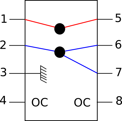
A height ports ideal junction
Each wire can be in one of three states :
- Connected to another wire (black circle)
- Connected to the ground (short-circuit)
- Not connected at all (open-circuit - OC)
The state set can be sum up in a (n x n) integer matrix C looking like :
| X | 1 | 2 | 3 | 4 | 5 | 6 | 7 | 8 |
|---|---|---|---|---|---|---|---|---|
| 1 | 0 | 0 | 0 | 0 | 1 | 0 | 0 | 0 |
| 2 | 0 | 0 | 0 | 0 | 0 | 1 | 1 | 0 |
| 3 | 0 | 0 | 1 | 0 | 0 | 0 | 0 | 0 |
| 4 | 0 | 0 | 0 | -1 | 0 | 0 | 0 | 0 |
| 5 | 1 | 0 | 0 | 0 | 0 | 0 | 0 | 0 |
| 6 | 0 | 1 | 0 | 0 | 0 | 0 | 1 | 0 |
| 7 | 0 | 1 | 0 | 0 | 0 | 1 | 0 | 0 |
| 8 | 0 | 0 | 0 | 0 | 0 | 0 | 0 | -1 |
The matrix’ elements are set up with the following rules :
Diagonal elements
- If C(i,i) = 1, the port i is connected to the ground
- If C(i,i) = -1, the port i is an open-circuit
- If C(i,i) = 0, the port is in the default state : not connected to the ground and not an open-circuit. It is connected to some ports
Non diagonal elements
- If C(i,j) = 1, the port i is connected to the port j
- If C(i,j) = 0, the port i is not connected to the port j
In Amelet-HDF, an ideal junction is a number port dimension
floatingType=dataSet defined by :
- A
typeattribute equals toidealJunction - Integer values, values are defined by the rules above.
Examples :
data.h5
`-- physicalModel/
    `-- multiport/
        `-- connection
            `-- $ideal_junction[@type=idealJunction
                                @floatingType=dataSet]
9.7. Distributed Multiport
/physicalModel/multiport/distributed contains transmission line distributed
parameters, i.e the RLCG matrices components. Those parameters are :
- distributed impedance
- distributed admittance
- distributed resistance
- distributed inductance
- distributed capacitance
- distributed conductance
A distributed multiport is a floatingType child
of /physicalModel/multiport/distributed with a mandatory attribute :
/physicalModel/multiport/distributed are expressed in the same way as
/physicalModel/multiport, except that the unit is :
ohmPerMeterforimpedancesiemensPerMeterforadmittanceohmPerMeterforresistancehenryPerMeterforinductancefaradPerMeterforcapacitancesiemensPerMeterforconductance
All children of these categories can be expressed by :
- A complex number
- A complex dataSet
- An array of complex numbers
- Some rational functions
Example
data.h5
`-- physicalModel/
    `-- multiport/
        `-- distributed
            |-- $disImp1[@floatingType=singleComplex
            |            @physicalNature=impedance
            |            @unit=ohmPerMeter
            |            @value=(10,2)]
            |-- $disImp2[@floatingType=dataSet
            |            @physicalNature=impedance
            |            @unit=ohmPerMeter]
            `-- $disImp3[@floatingType=arraySet]
                |-- data[@physicalNature=impedance
                |        @unit=ohmPerMeter]
                `-- ds
                    `-- dim1[@physicalNature=frequency]
9.8. Surface
This section describes surface material models, we can see two main types detailed in the next sections :
- the thin dielectric layer model
- the surface impedance boundary condition model
Model or genuine surface, instances can have a physicalModel attribute
which gives the volume characteristics of the material.
Example
data.h5
`-- physicalModel/
    |-- volume/
    |   `-- $mat1
    `-- surface/
        `-- $layer[@type=XXX
                   @physicalModel=/physicalModel/volume/$mat1]
9.8.1. Thin dielectric layer
The thin dielectric layer represents a dielectric layer thinner than the cell dimension. Surface impedance boundary models are not used to make wave propagate through the panel but the equivalent medium is computed from the weighting of the layer characteristics and the surrounding medium properties.
Example
data.h5
`-- physicalModel/
    |-- volume/
    |   `-- $mat1
    `-- surface/
        `-- $layer[@type=thinDielectricLayer
                   @physicalModel=/physicalModel/volume/$mat1
                   @thickness=1e-3]
9.8.2. SIBC
The thin dielectric layer represents a dielectric layer thiner than the cell dimension. Surface impedance boundary models are used to make wave propagate through the panel, the surface impedance is computed by the solver.
Example
data.h5
`-- physicalModel/
    |-- volume/
    |   `-- $mat1
    `-- surface/
        `-- $layer[@type=SIBC
                   @physicalModel=/physicalModel/volume/$mat1
                   @thickness=1e-3]
9.8.3. Zs
The thin dielectric layer represents a dielectric layer thiner than the cell dimension. Surface impedance boundary models are used to make wave propagate through a panel and the surface impedance is given by the model.
The relation between \(\overrightarrow{E}\) and \(\overrightarrow{H}\) is :
\(\overrightarrow{J}\) is the surface current vector.
Example
data.h5
`-- physicalModel/
    |-- volume/
    |   `-- $mat1
    |-- multiport/
    |   `-- $Zs[@floatingType=rational
    |       |   @physicalNature=impedance]
    |       |-- function
    |       |   |-- $Z11[@floatingType=generalRationalFunction
                         @type=polynomial]
    |       |   `-- $Z12[@floatingType=generalRationalFunction
                         @type=partialFraction]
    |       `-- data
    `-- surface/
        `-- $layer[@type=Zs
                   @Zs=/physicalModel/multiport/$Zs
                   @physicalModel=/physicalModel/volume/$mat1]
with data.h5:/physicalModel/multiport/Zs/function/Z11 :
| (5.9545e69, 0) | (2.9773e69, 0) |
| (9.0191e59, 0) | (1.3921e59, 0) |
| (1.9344e49, 0) | (1.6254e48, 0) |
| (1.3458e38, 0) | (7.0897e36, 0) |
| (3.7609e26, 0) | (1.2717e26, 0) |
| (4.2033e14, 0) | (8.3344e05, 0) |
| (138.73, 0) | (1., 0) |
with data.h5:/physicalModel/multiport/Zs/function/Z12 :
| degree | A | B |
|---|---|---|
| 1 | (50, 0) | (0.5e-9, 4) |
| 2 | (125, 12.5) | (-15.25, 4) |
| 1 | (1.e9, 0) | (31, 0) |
with data.h5:/physicalModel/multiport/Zs/data :
| $Z11 | $Z12 |
| $Z21 | $Z11 |
9.8.4. ZsZt
The thin dielectric layer represents a dielectric layer thiner than the cell dimension. Surface impedance boundary models are used to make wave propagate through the panel, Zs and Zt are given by the model.
Example
data.h5
`-- physicalModel/
    |-- volume/
    |   `-- $mat1
    |-- multiport/
    |   |-- $Zs[@physicalNature=impedance]
    |   `-- $Zt[@physicalNature=impedance]
    `-- surface/
        `-- $layer[@type=ZsZt
                   @Zs=/physicalModel/multiport/$Zs
                   @Zt=/physicalModel/multiport/$Zt
                   @physicalModel=/physicalModel/volume/$mat1]
9.8.5. ZsZt2
The thin dielectric layer represents a dielectric layer thiner than the cell dimension. Surface impedance boundary models are used to make wave propagate through the panel, Zs and Zt are given by the model. Front face (1) and back face (2) have different behavior.
Example
data.h5
`-- physicalModel/
    |-- volume/
    |   `-- $mat1
    |-- multiport/
    |   |-- $Zs1[@physicalNature=impedance]
    |   |-- $Zs2[@physicalNature=impedance]
    |   |-- $Zt1[@physicalNature=impedance]
    |   `-- $Zt2[@physicalNature=impedance]
    `-- surface/
        `-- $layer[@type=ZsZt2
                   @Zs1=/physicalModel/multiport/$Zs1
                   @Zt1=/physicalModel/multiport/$Zt1
                   @Zs2=/physicalModel/multiport/$Zs2
                   @Zt2=/physicalModel/multiport/$Zt2
                   @physicalModel=/physicalModel/volume/$mat1]
9.9. Interface
Objects contained in the category /physicalModel/interface
define the connection between
two media. An interface is a named HDF5 group with two mandatory attributes
and one optional attribute :
Mandatory attributes :
medium1is an HDF5 string attribute, it is a pointer to a/physicalModel, first medium of the interfacemedium2is an HDF5 string attribute, it is a pointer to a/physicalModel, second medium of the interface
Optional attribute :
interfaceis an HDF5 string attribute, it is a pointer to a/physicalModel, it represents the properties of the interface (infinitely thin, or not meshed).
Below is an example of an interface separating two areas made up of
/physicalModel/volume/$diel1 and /physicalModel/volume/$diel2.
The interface itself (virtual space between the two media) is an infinitely
thin perfectly conducting plane.
data.h5
`-- physicalModel/
    |-- volume
    |   |-- $diel1
    |   `-- $diel2
    `-- interface/
        `-- $interface1[@medium1=/physicalModel/volume/$diel1
                        @medium2=/physicalModel/volume/$diel2
                        @interface=/physicalModel/perfectElectricConductor]
9.10. Aperture
In the electromagnetic simulation domain,
little aperture are often described thanks to
sub cellular models associated to linear elements,
they don’t appear in the mesh as slot
but as linear elements. In addition, apertures can be filled (loaded) by a
materialModel.
An aperture is a named HDF5 group child of /physicalModel/aperture
that have a type attribute. The type
is a string HDF5 attribute.
Amelet HDF defines three apertures that are described in the next sections :
- Slot
- Rectangular aperture
- Circular aperture
- Elliptic aperture
- Large aperture
- Measured aperture
9.10.1. Slot
A slot is a named HDF5 group with type equals slot, it has three
attributes :
witdh: the width of the slot, a length in meter, it is a float HDF5 attribute and is mandatory.thickness: the thickness of the slot, a length in meter, it is a float HDF5 attribute and is mandatory.materialModel: the load material name of the slot, it is a character strings, it is optional.
Example :
data.h5
`-- physicalModel/
    |-- volume/
    |   `-- $diel1
    `-- aperture/
        `-- $slot1[@type=slot
                   @width=10e-3
                   @thickness=2e-3
                   @materialModel=/physicalModel/volume/$diel1]
9.10.2. Rectangular aperture
A rectangular aperture is a named HDF5 group with type equals
rectangular, it has two attributes :
length: the length of the rectangle, a length in meter, it is a float HDF5 attribute and is mandatory.width: the width of the rectangle, a length in meter, it is a float HDF5 attribute and is mandatory.thickness: the thickness of the aperture, a length in meter, it is a float HDF5 attribute and is mandatory.materialModel: the load material name of the aperture, it is a character strings, it is optional.
Example :
data.h5
`-- physicalModel/
    |-- volume/
    |   `-- $diel1
    `-- aperture/
        `-- $rectangularAperture1[@type=rectangular
                                  @length=10e-3
                                  @width=6e-3
                                  @thickness=2e-3
                                  @materialModel=/physicalModel/volume/$diel1]
9.10.3. Circular aperture
A circular aperture is a named HDF5 group with type equals circular,
it has two attributes :
diameter: the diameter of the circle, a length in meter, it is a float HDF5 attribute and is mandatory.thickness: the thickness of the aperture, a length in meter, it is a float HDF5 attribute and is mandatory.materialModel: the load material name of the aperture, it is a character strings, it is optional.
Example :
data.h5
`-- physicalModel/
    |-- volume/
    |   `-- $diel1
    `-- aperture/
        `-- $circularAperture1[@type=circular
                               @diameter=10e-3
                               @thickness=2e-3
                               @materialModel=/physicalModel/volume/$diel1]
9.10.4. Elliptic aperture
A elliptic aperture is a named HDF5 group with type equals Elliptic,
it has two attributes :
semimajorAxis: the semimajor axis of the ellipse, a length in meter, it is a float HDF5 attribute and is mandatory.semiminorAxis: the semiminor axis of the ellipse, a length in meter, it is a float HDF5 attribute and is mandatory.thickness: the thickness of the aperture, a length in meter, it is a float HDF5 attribute and is mandatory.materialModel: the load material name of the aperture, it is a character strings, it is optional.
Example :
data.h5
`-- physicalModel/
    |-- volume/
    |   `-- $diel1
    `-- aperture/
        `-- $ellipticAperture1[@type=elliptic
                               @semimajorAxis=10e-3
                               @semiminorAxis=6e-3
                               @thickness=2e-3
                               @materialModel=/physicalModel/volume/$diel1]
9.10.5. Large aperture
A large aperture relative to the wave length is a named HDF5 group
with type equals large, it has three attribute :
surface: the surface of the aperture, a surface in square meter, it is a float HDF5 attribute and is mandatory.thickness: the thickness of the aperture, a length in meter, it is a float HDF5 attribute and is mandatory.materialModel: the load material name of the aperture, it is a character strings, it is optional.
Example :
data.h5
`-- physicalModel/
    |-- volume/
    |   `-- $diel1
    `-- aperture/
        `-- $largeAperture1[@type=large
                            @surface=10e-3
                            @thickness=2e-3
                            @materialModel=/physicalModel/volume/$diel1]
9.10.6. Measured aperture
A measured aperture is a named HDF5 group with type equals measured,
it has one floatingType child called sigma. sigma is the
measured transmission cross section as function of incident field
and frequency.
Example :
data.h5
`-- physicalModel/
    `-- aperture/
        `-- $measuredAperture1[@type=measured]
            `-- sigma[@floatingType=arraySet]
                |-- data[@physicalNature=surface
                |        @unit=squareMeter]
                `-- ds/
                    `-- dim1[@physicalNature=frequency
                             @unit=hertz]
9.11. Shield
The shield category contains shields definitions.
9.11.1. Metal braid shield
A metal braid is a shield for a cable or for a bundle of cables :
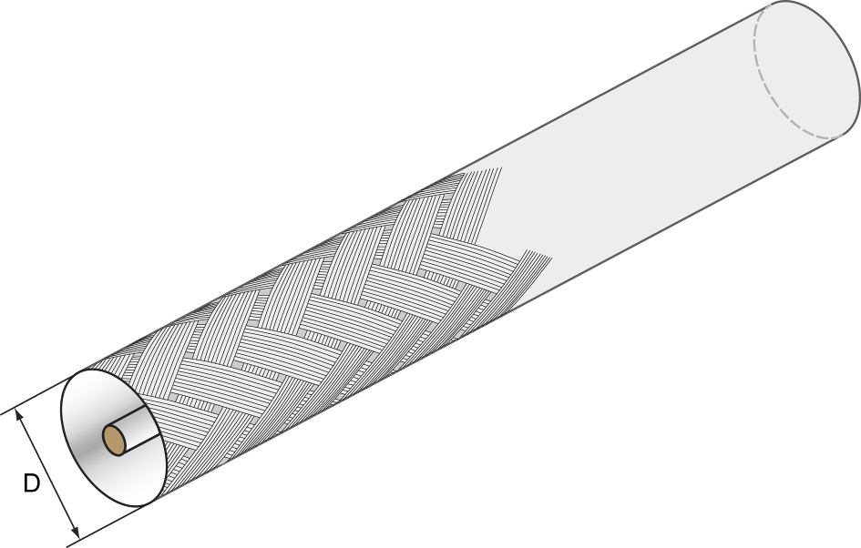
Metal braid representation
A metal braid is completely described by six parameters :
- Diameter D (real number, dimension meters)
- Number of carriers C (i.e. belts of wires) in the braid (integer number)
- Number of wires N in a carrier (integer number)
- Diameter d of a single wire (real number, dimension meters)
- Conductivity \(\sigma\) of the wires (real number, dimension Simens per meters)
- Weave angle \(\alpha\) (real number, degrees)
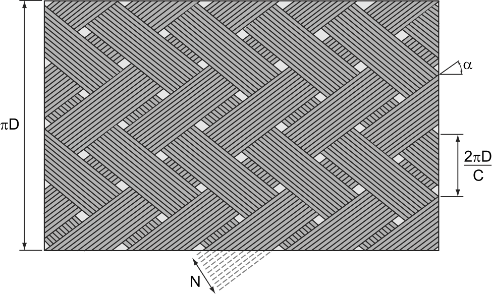
Metal braid chracteristics
In Amelet HDF a metal braid is an HDF5 named group with seven attributes :
type:typeis an HDF5 string attribute, its value ismetalBraidbraidDiameter:braidDiameteris an HDF5 real attribute and represents D in metersnumberOfCarriers:numberOfCarriersis an HDF5 integer attribute and is the number of carriers C.numberOfWiresPerCarrier:numberOfWiresPerCarrieris an HDF5 integer attribute and represents the number of wires N in a carrierwireDiameter:wireDiameteris an HDF5 real attribute and represents d in metersmaterial:materialis an HDF5 string attribute, it contains the name of a/physicalModel/volumematerialweaveAngle:weaveAngleis an HDF5 real number which represents the angle \(\alpha\) in degrees
and a floatingType child named Zt. Zt contains
the transfer impedance of the shield.
Example :
data.h5
`-- physicalModel/
    |-- volume/
    |   `-- $copper
    |       `-- electricConductivity[@floatingType=singleReal
    |                                @value=59.6e6]
    `-- shield/
        `-- $a-metal-braid[@type=metalBraid
            |              @braidDiameter=5e-3
            |              @numberOfCarriers=10
            |              @numberOfWiresPerCarrier=20
            |              @wireDiameter=5e-4
            |              @material=/physicalModel/volume/$copper
            |              @weaveAngle=45]
            `-- Zt[@floatingType=arraySet]
                |-- data
                `-- ds
                    `-- dim1
9.12. Grid
The grid category contains grids definition. Many kinds of grid exist.
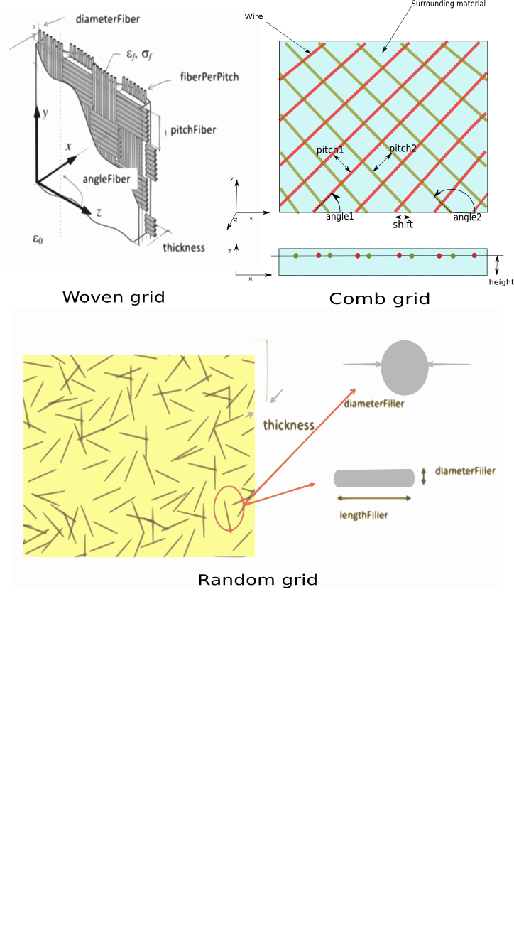
Grids characteristics
A grid is composed of two materials:
- The grid itself
- A material around the grid
A grid is defined by many parameters:
- Physical characteristics of the surrounding material
- Physical characteristics of the grid
- Dimension of the grid’s wires for woven and comb grids
(real number in meters):
- Diameter if wires have a circular section
- Thickness and width if wires have a rectangular section
- Texture type (woven, unidirectional, comb, random)
There are specific parameters to describe each kind of grid.
- A woven/unidirectional grid is defined by:
- Number of fiber per pitch (integer number)
- Length of a pitch (real number in meters)
- Angle between the fiber and the Z-axis (real number in degrees)
- Model type homgeneous or heterogeneous composite
- A comb grid is defined by:
- Angles relative to the X-axis (real number in degrees)
- Pitches, distances between two wire centers (real number in meters)
- Height of the grid from the bottom (z=0) in the context of layer
- Model type homgeneous or heterogeneous composite
- A random grid:
- Scale filler : micro or nano (string)
- Type filler : sphere, rod or disk (string)
- Volume fraction of filler (real number)
- Diameter of filler (real number in meter)
- Length of filler (real number in meter)
In Amelet HDF a grid is an HDF5 named group with the following attributes :
surroundingMaterial:surroundingMaterialis an HDF5 string attribute, it contains the name of a/physicalModel/volumematerial.gridMaterial:gridMaterialis an HDF5 string attribute, it contains the name of a/physicalModel/volumematerial.textureType:textureTypeis an HDF5 string attribute and defines the type of grid texture. The accepted values arewoven,unilateral,combandrandom.pitchFiber:pitchFiberis an optional HDF5 real attribute, it represents the length of a pitch. This attribute is present iftextureTypeis equal towoven.fiberPerPitch:fiberPerPitchis an optional HDF5 integer attribute, it represents the number of fiber per pitch. This attribute is present iftextureTypeis equal towoven.wireSectionType:wireSectionTypeis an HDF5 string attribute and defines the type of the wire. The accepted values arecircularorrectangular.diameterWire:diameterWireis an optional HDF5 real attribute and represents the grid’s wire diameter in meters. This attribute is present ifwireSectionTypeis equal tocircularor iftextureTypeis equal torandom.thicknessWire:thicknessWireis an optional HDF5 real attribute and represents the grid’s wire thickness in meters. This attribute is present ifwireSectionTypeis equal torectangular.widthWire:widthWireis an optional HDF5 real attribute and represents the grid’s wire width in meters. This attribute is present ifwireSectionTypeis equal torectangular.lengthWire:lengthWireis an optional HDF5 real attribute and represents the length of wire in meter which fills the material. This attribute is present iftextureTypeis equal torandom.scaleFiller:scaleFilleris an optional HDF5 string attribute and represents the scale filled of the material. This attribute can have only two possible valuesmicroornano.typeFiller:typeFilleris an optional HDF5 string attribute and represents the filled type of the material. This attribute can have only three possible valuessphere,rodornano.volFractioFiller:volFractioFilleris an optional HDF5 real attribute and represents the ratio of filling volume.shift:shiftis the optional distance in meters between the two combs measured on the X-axis (see the sketch).modelType:modelTypeis the optional HDF5 string attribute and represents the kind of material. Value can be homogeneous or heterogeneous.
and one or two HDF5 group named comb1 (and optionally comb2 if
there are two combs) with attributes as follows :
- Height of the grid from the bottom (z=0) of a layer :
relativeHeightrepresents a relative height relative to the total height of a material layer. It is a dimensionless float between 0 and 1absoluteHeightrepresents an absolute height from the bottom of a material layer. It is a float number in meters.
pitch:pitchis an HDF5 real attribute and represents the distance between two wire centers in metersangle:angleis an HDF5 real attribute and represents the angle in degrees between wires and the X-axis.
Example of a woven Grid with a thickness of 5 mm :
data.h5
`-- physicalModel/
    |-- multilayer/
    |   `-- $multilayerMaterial
    |-- volume/
    |   |-- $resin
    |   |   |-- electricConductivity[@floatingType=singleReal
    |   |   |                        @value=0.0]
    |   |   |-- magneticConductivity[@floatingType=singleReal
    |   |   |                        @value=0.0]
    |   |   |-- relativePermittivity[@floatingType=singleReal
    |   |   |                        @value=2.0]
    |   |   `-- relativePermeability[@floatingType=singleReal
    |   |                            @value=1.0]
    |   `-- $fiber
    |       |-- electricConductivity[@floatingType=singleReal
    |       |                        @value=1.0e5]
    |       |-- magneticConductivity[@floatingType=singleReal
    |       |                        @value=0.0]
    |       |-- relativePermittivity[@floatingType=singleReal
    |       |                        @value=2.0]
    |       `-- relativePermeability[@floatingType=singleReal
    |                                @value=1.0]
    `-- grid/
        `-- $a-wovengrid[@surroundingMaterial=/physicalModel/volume/$resin
             |           @gridMaterial=/physicalModel/volume/$fiber
             |           @textureType=woven
             |           @pitchFiber=0.1e-3
             |           @fiberPerPitch=10
             |           @modelType=homogeneous]
             `-- comb1[@relativeHeight=0.5
                       @angle=90.0
                       @diameterWire=2.5e-5
                       @wireSectionType=circular]
$multilayerMaterial is a table which contains:
| physicalModel | thickness |
|---|---|
/physicalModel/grid/$a-wovengrid |
5.0e-3 |
Example of a two single comb Grid with a thickness of 3 mm :
data.h5
`-- physicalModel/
    |-- multilayer/
    |   `-- $multilayerMaterial
    |-- volume/
    |   |-- $resin
    |   |   |-- electricConductivity[@floatingType=singleReal
    |   |   |                        @value=0.0]
    |   |   |-- magneticConductivity[@floatingType=singleReal
    |   |   |                        @value=0.0]
    |   |   |-- relativePermittivity[@floatingType=singleReal
    |   |   |                        @value=2.0]
    |   |   `-- relativePermeability[@floatingType=singleReal
    |   |                            @value=1.0]
    |   `-- $fiber
    |       |-- electricConductivity[@floatingType=singleReal
    |       |                        @value=1.0e5]
    |       |-- magneticConductivity[@floatingType=singleReal
    |       |                        @value=0.0]
    |       |-- relativePermittivity[@floatingType=singleReal
    |       |                        @value=2.0]
    |       `-- relativePermeability[@floatingType=singleReal
    |                                @value=1.0]
    `-- grid/
        `-- $a-combgrid[@surroundingMaterial=/physicalModel/volume/$resin
             |          @gridMaterial=/physicalModel/volume/$fiber
             |          @textureType=comb
             |          @shift=0.3e-4
             |          @modelType=heterogeneous]
             |-- comb1[@relativeHeight=0.5
             |         @angle=45.0
             |         @pitch=1.0e-4
             |         @thicknessWire=2.5e-5
             |         @widthWire=5.0e-5
             |         @wireSectionType=rectangular]
             `-- comb2[@relativeHeight=0.4
                       @angle=135.0
                       @pitch=1.0e-4
                       @thicknessWire=2.5e-5
                       @widthWire=5.0e-5
                       @wireSectionType=rectangular]
$multilayerMaterial is a table which contains:
| physicalModel | thickness |
|---|---|
/physicalModel/grid/$a-combgrid |
3.0e-3 |
Example of a random Grid with a thickness of 4 mm and three kind of wire:
data.h5
`-- physicalModel/
    |-- multilayer/
    |   `-- $multilayerMaterial
    |-- volume/
    |   |-- $resin
    |   |   |-- electricConductivity[@floatingType=singleReal
    |   |   |                        @value=0.0]
    |   |   |-- magneticConductivity[@floatingType=singleReal
    |   |   |                        @value=0.0]
    |   |   |-- relativePermittivity[@floatingType=singleReal
    |   |   |                        @value=2.0]
    |   |   `-- relativePermeability[@floatingType=singleReal
    |   |                            @value=1.0]
    |   |-- $fiber1
    |   |   |-- electricConductivity[@floatingType=singleReal
    |   |   |                        @value=1.5e5]
    |   |   |-- magneticConductivity[@floatingType=singleReal
    |   |   |                        @value=0.0]
    |   |   |-- relativePermittivity[@floatingType=singleReal
    |   |   |                        @value=1.0]
    |   |   `-- relativePermeability[@floatingType=singleReal
    |   |
    |   `-- $fiber2
    |       |-- electricConductivity[@floatingType=singleReal
    |       |                        @value=1.0e5]
    |       |-- magneticConductivity[@floatingType=singleReal
    |       |                        @value=0.0]
    |       |-- relativePermittivity[@floatingType=singleReal
    |       |                        @value=1.0]
    |       `-- relativePermeability[@floatingType=singleReal
    |                                @value=1.0]
    `-- grid/
        `-- $a-randomgrid[@surroundingMaterial=/physicalModel/volume/$resin
            |             @textureType=random]
            |-- a-nano-filler[@gridMaterial=/physicalModel/volume/$fiber1
            |                 @scaleFiller=nano
            |                 @typeFiller=rod
            |                 @volFractioFiller=0.1
            |                 @diameterWire=1.e-9
            |                 @lengthWire=5.0e-8]
            |-- a-micro-filler[@gridMaterial=/physicalModel/volume/$fiber2
            |                  @scaleFiller=micro
            |                  @typeFiller=rod
            |                  @volFractioFiller=0.2
            |                  @diameterWire=1.e-5
            |                  @lengthWire=5.0e-5]
            `-- another-micro-filler[@gridMaterial=/physicalModel/volume/$fiber2
                                     @scaleFiller=micro
                                     @typeFiller=rod
                                     @volFractioFiller=0.05
                                     @diameterWire=0.5e-6
                                     @lengthWire=1.0e-5]
$multilayerMaterial is a table which contains:
| physicalModel | thickness |
|---|---|
/physicalModel/grid/$a-randomgrid |
4.0e-3 |