6. Mesh
Computer simulations work well using a discretized space, this discretization of the space is the result of the mesh generation process of a CAD model.
Over-all the mesh data structure is made up of three kinds of elements :
- the nodes. The nodes are points in space and are the foundations of the mesh.
- the elements. The elements are geometrical shapes connecting neighboring nodes.
- the groups. The groups are sets of elements and represent areas, volumes that are important for the simulation.
A mesh can be either structured or unstructured.
6.1. The Mesh category
In Amelet HDF meshes are localized in the /mesh category
and can be named by whatever word authorized by HDF5, its
children are mesh groups.
6.1.1. Mesh group
Meshes are gathered inside “mesh groups”. In fact, meshes are often made up of independent mesh part, like hybrid meshes for instance. (An hybrid mesh is mesh composed of unstructured meshes and structured meshes).
A mesh group is named HDF5 group.
(see the data.h5:/mesh/$gmesh1 group below)
Consequently, the name of the system is rather the group’s name rather than the mesh name.
Example :
data.h5/
`-- mesh/
    |-- $gmesh1/
    `-- $gmesh2/
6.1.2. Mesh
Meshes are children of mesh groups with a mandatory attribute : type.
type can take the following values :
unstructured: the mesh is an unstructured mesh.structured: the mesh is an structured mesh.
Mesh’s name and mesh group’ name must have a length inferior to 20 characters.
Example of a /mesh category :
data.h5/
`-- mesh/
    |-- $gmesh1
    |    |-+ $mesh#5
    |    `-+ $mesh_6
    `-- $gmesh2
        |-- $mesh1[@type=unstructured]/
        |   |-- elementNodes
        |   |-- elementTypes
        |   |-- nodes
        |   |-- group
        |   |   |-- $field-location[@type=node]
        |   |   |-- $right-wing[@type=face]
        |   |   `-- $left-wing[@type=face]
        |   |-- groupGroup
        |   |   `-- $wings
        |   `-- selectorOnMesh
        |       |-- nodes
        |       |-- elements
        |       `-- groups
        |-+ $mesh-two
        `-- $mesh-3[@type=structured]/
            |-- cartesianGrid
            |-- group
            |   |-- $field-location[@type=node]
            |   |-- $right-wing[@type=face]
            |   `-- $left-wing[@type=face]
            |-- groupGroup
            |   `-- $wings
            `-- selectorOnMesh
                |-- nodes
                |-- elements
                `-- groups
In this example, data.h5:/mesh/$gmesh2/$mesh1 is an unstructured mesh and
data.h5:/mesh/gmesh2/$mesh-3 is a structured mesh.
The next section present in details unstructured mesh and structured
meshes.
6.2. Unstructured mesh
An unstructured mesh is a mesh based upon nodes dispatched in the space. Nodes are connected together by edges to form the mesh elements. Mesh elements can be :
- Line or 1d : edge
- Surface or 2d : triangle, quadrilateral, polygon ...
- Volume or 3d : tetrahedron, cube ...
Then elements are gathered to create groups of importance for the simulation. A group can represent a plane wing, a wheel, a dipole, a wire antenna, an output request location.
A mesh is a named group child of the /mesh group. A mesh mainly comprises
three datasets :
- The nodes dataset
- The nodes dataset contains the definition (x, y, z in 3d) of all nodes
- The elementTypes dataset
- The elementTypes dataset contains the definition of the type of the mesh elements
- The elements dataset
- The elements dataset contains the linked node’s indices for all elements
Example :
data.h5
`-- mesh/
    `-- $gmesh1
        `-- mesh1[@type=unstructured]/
            |-- nodes
            |-- elementTypes
            `-- elementNodes
6.2.1. Attributes
The value of the attribute type of an unstructured mesh is unstructured.
6.2.2. nodes
All mesh nodes are defined in the /mesh/$gmesh/$mesh/nodes dataset.
A node is defined by one to three coordinates :
xin a 1d spacex,yin a 2d spacex,yandzin 3d space
x, y, z are real numbers.
The nodes dataset is a two dimensional real dataset, its dimensions are
(number_of_nodes x number_of_space_dimensions).
The first column is x, the second is y and the third is z. The index of a node is the row’s index in which it appears.
The index and columns header are implicit. The index starts at 0.
| i | x | y | z |
|---|---|---|---|
| 0 | 0.0 | 0.0 | 0.0 |
| 1 | 0.0 | 1.0 | 0.0 |
| 2 | 1.0 | 0.0 | 2.0 |
Here, three nodes are defined in a 3d space, the genuine dataset without headers is :
| 0.0 | 0.0 | 0.0 |
| 0.0 | 1.0 | 0.0 |
| 1.0 | 0.0 | 2.0 |
6.2.3. elementTypes
6.2.3.1. Explicit nodal approach
The elements of an unstructured mesh are defined by the nodal approach, that is to say that each element is defined by a set of nodes. For a given number of nodes, many geometric shapes are possible, then each shape has a type and the shape’s type is the element’s type.
Warning
Nodes are numbered and numbers are important for element definition and normal computation.
6.2.3.2. Implicit sub-element
In addition this section introduces the definition of (implicit) sub-elements
(edges for entityType=face, edges and faces for entityType=volume) of
an element, these sub-elements are numbered as well. Implicit sub-elements
permit to select (n-1) dimensional sub-elements of an n dimensional element.
Warning
Implicit edges and faces are numbered.
Implicit sub-elements can be seen as the way to make a link with the mesh definition by the descendant approach (node, edge, face, volume) .
6.2.3.3. Predefined shapes types
The predefined shape types are detailed in the following sections.
Note
Node numbers are shown in black, edge numbers in red and face number in blue.
6.2.3.3.1. bar2
bar2 cell characteristics are :
- one-dimensional cell
- 2 nodes
- 1 edge
- code : 1
Edges are (defined by nodes) :
| Edge number | Node 1 | Node 2 |
|---|---|---|
| 1 | 1 | 2 |
The following figure shows a bar2 cell :
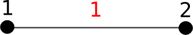
A bar2 cell
6.2.3.3.2. bar3
bar3 cell characteristics are :
- one-dimensional cell
- 3 nodes
- 2 edges
- code : 2
- comment : 1 node is in the middle of the edge defined by the two endpoints
Edges are (defined by nodes) :
| Edge number | Node 1 | Node 2 |
|---|---|---|
| 1 | 1 | 3 |
| 2 | 3 | 2 |
The following figure shows a bar3 cell :
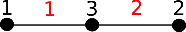
A bar3 cell
6.2.3.3.3. tri3
tri3 cell characteristics are :
- two-dimensional cell
- 3 nodes
- 3 edges connecting all nodes each other and 1 face.
- code : 11
Edges are (defined by nodes) :
| Edge number | Node 1 | Node 2 |
|---|---|---|
| 1 | 1 | 2 |
| 2 | 2 | 3 |
| 3 | 3 | 1 |
Faces are (defined by nodes) :
| Face number | Node 1 | Node 2 | Node 3 |
|---|---|---|---|
| 1 | 1 | 2 | 3 |
The following figure shows a tri3 cell :
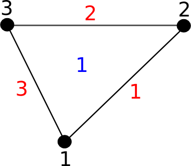
A tri3 cell
6.2.3.3.4. tri6
tri6 cell characteristics are :
- two-dimensional cell
- 6 nodes
- 6 edges
- 1 face
- code : 12
- comment : 3 nodes are in the middle of the edges
Edges are (defined by nodes) :
| Edge number | Node 1 | Node 2 |
|---|---|---|
| 1 | 1 | 4 |
| 2 | 4 | 2 |
| 3 | 2 | 5 |
| 4 | 5 | 3 |
| 5 | 3 | 6 |
| 6 | 6 | 1 |
Faces are (defined by nodes) :
| Face number | Node 1 | Node 2 | Node 3 |
|---|---|---|---|
| 1 | 1 | 2 | 3 |
The following figure shows a tri6 cell :
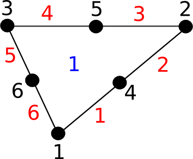
A tri6 cell
6.2.3.3.5. quad4
quad4 cell characteristics are :
- two-dimensional cell
- 4 nodes
- 4 edges
- 1 face
- code : 13
Edges are (defined by nodes) :
| Edge number | Node 1 | Node 2 |
|---|---|---|
| 1 | 1 | 2 |
| 2 | 2 | 3 |
| 3 | 3 | 4 |
| 4 | 4 | 1 |
Faces are (defined by nodes) :
| Face number | Node 1 | Node 2 | Node 3 | Node 4 |
|---|---|---|---|---|
| 1 | 1 | 2 | 3 | 4 |
The following figure shows a quad4 cell :
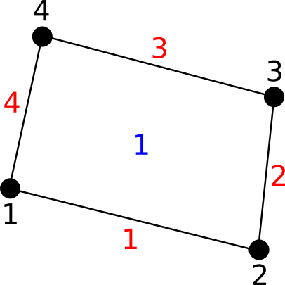
A quad4 cell
6.2.3.3.6. quad8
quad8 cell characteristics are :
- two-dimensional cell
- 8 nodes
- 4 edges
- 1 face
- code : 14
- comment : 4 nodes in the middle of the edges
Edges are (defined by nodes) :
| Edge number | Node 1 | Node 2 |
|---|---|---|
| 1 | 1 | 5 |
| 2 | 5 | 2 |
| 3 | 2 | 6 |
| 4 | 6 | 3 |
| 5 | 3 | 7 |
| 6 | 7 | 4 |
| 7 | 4 | 8 |
| 8 | 8 | 1 |
Faces are (defined by nodes) :
| Face number | Node 1 | Node 2 | Node 3 | Node 4 |
|---|---|---|---|---|
| 1 | 1 | 2 | 3 | 4 |
The following figure shows a quad8 cell :
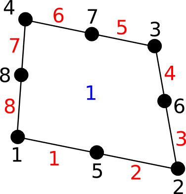
A quad8 cell
6.2.3.3.7. tetra4
tetra4 cell characteristics are :
- three-dimensional cell
- 4 nodes
- 6 edges connecting all node each other
- 4 faces
- code : 101
Edges are (defined by nodes) :
| Edge number | Node 1 | Node 2 |
|---|---|---|
| 1 | 1 | 2 |
| 2 | 2 | 3 |
| 3 | 3 | 1 |
| 4 | 1 | 4 |
| 5 | 2 | 4 |
| 6 | 3 | 4 |
Faces are (defined by nodes) :
| Face number | Node 1 | Node 2 | Node 3 |
|---|---|---|---|
| 1 | 1 | 2 | 4 |
| 2 | 2 | 3 | 4 |
| 3 | 1 | 4 | 3 |
| 4 | 1 | 3 | 2 |
The following figure shows a tetra4 cell :
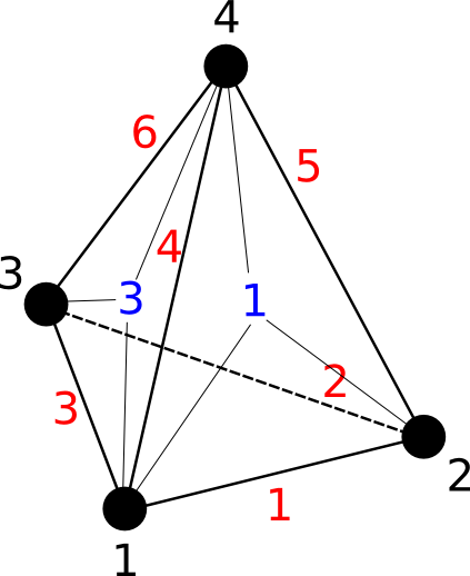
A tetra4 cell
6.2.3.3.8. pyra5
pyra5 cell characteristics are :
- three-dimensional cell
- 5 nodes
- 8 edges
- 5 faces
- code : 102
Edges are (defined by nodes) :
| Edge number | Node 1 | Node 2 |
|---|---|---|
| 1 | 1 | 2 |
| 2 | 2 | 3 |
| 3 | 3 | 4 |
| 4 | 4 | 1 |
| 5 | 1 | 5 |
| 6 | 2 | 5 |
| 7 | 3 | 5 |
| 8 | 4 | 5 |
Faces are (defined by nodes) :
| Face number | Node 1 | Node 2 | Node 3 | Node 4 |
|---|---|---|---|---|
| 1 | 1 | 4 | 3 | 2 |
| 1 | 1 | 2 | 5 | |
| 1 | 2 | 3 | 5 | |
| 1 | 3 | 4 | 5 | |
| 1 | 1 | 5 | 4 |
The following figure shows a pyra5 cell :
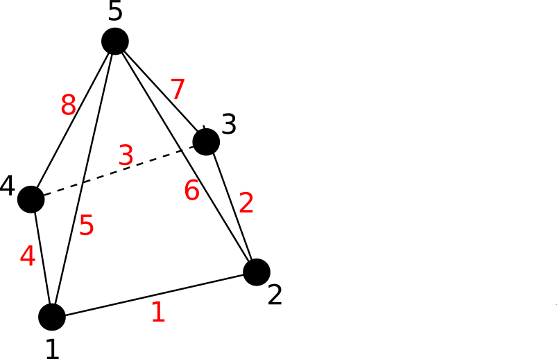
A pyra5 cell
6.2.3.3.9. penta6
penta6 cell characteristics are :
- three-dimensional cell
- 6 nodes
- 9 edges
- 5 faces
- code : 103
Edges are (defined by nodes) :
| Edge number | Node 1 | Node 2 |
|---|---|---|
| 1 | 1 | 2 |
| 2 | 2 | 5 |
| 3 | 5 | 4 |
| 4 | 4 | 1 |
| 5 | 1 | 3 |
| 6 | 2 | 3 |
| 7 | 4 | 6 |
| 8 | 5 | 6 |
| 9 | 3 | 6 |
Faces are (defined by nodes) :
| Face number | Node 1 | Node 2 | Node 3 | Node 4 |
|---|---|---|---|---|
| 1 | 1 | 4 | 5 | 2 |
| 2 | 1 | 2 | 3 | |
| 3 | 4 | 6 | 5 | |
| 4 | 2 | 5 | 6 | 3 |
| 5 | 1 | 3 | 6 | 4 |
The following figure shows a penta6 cell :
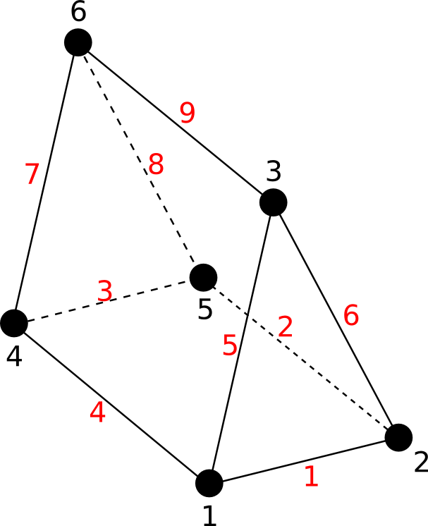
A penta6 cell
6.2.3.3.10. hexa8
hexa8 cell characteristics are :
- three-dimensional cell
- 8 nodes
- 12 edges
- 6 faces
- code : 104
Edges are (defined by nodes) :
| Edge number | Node 1 | Node 2 |
|---|---|---|
| 1 | 1 | 2 |
| 2 | 2 | 5 |
| 3 | 5 | 4 |
| 4 | 4 | 1 |
| 5 | 1 | 3 |
| 6 | 2 | 3 |
| 7 | 4 | 6 |
| 8 | 5 | 6 |
| 9 | 3 | 6 |
Faces are (defined by nodes) :
| Face number | Node 1 | Node 2 | Node 3 | Node 4 |
|---|---|---|---|---|
| 1 | 1 | 4 | 3 | 2 |
| 2 | 1 | 2 | 6 | 5 |
| 3 | 2 | 3 | 7 | 6 |
| 4 | 3 | 4 | 8 | 7 |
| 5 | 1 | 5 | 8 | 4 |
| 6 | 5 | 6 | 7 | 8 |
The following figure shows a hexa8 cell :
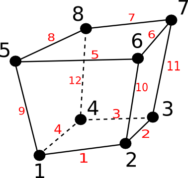
A hexa8 cell
6.2.3.3.11. tetra10
tetra10 cell characteristics are :
- three-dimensional cell
- 10 nodes
- 12 edges connecting all node each other
- 4 faces
- code : 108
Edges are (defined by nodes) :
| Edge number | Node 1 | Node 2 |
|---|---|---|
| 1 | 1 | 2 |
| 2 | 2 | 3 |
| 3 | 3 | 1 |
| 4 | 1 | 4 |
| 5 | 2 | 4 |
| 6 | 3 | 4 |
Faces are (defined by nodes) :
| Face number | Node 1 | Node 2 | Node 3 |
|---|---|---|---|
| 1 | 1 | 2 | 4 |
| 2 | 2 | 3 | 4 |
| 3 | 1 | 4 | 3 |
| 4 | 1 | 3 | 2 |
The following figure shows a tetra10 cell :
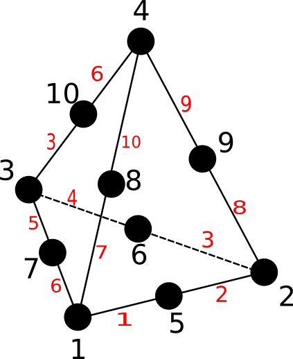
A tetra10 cell
6.2.3.3.12. hexa20
hexa20 cell characteristics are :
- three-dimensional cell
- 20 nodes
- 24 edges connecting all node each other
- 4 faces
- code : 109
Edges are (defined by nodes) :
| Edge number | Node 1 | Node 2 |
|---|---|---|
| 1 | 1 | 9 |
| 2 | 9 | 2 |
| 3 | 2 | 10 |
| 4 | 10 | 3 |
| 5 | 3 | 11 |
| 6 | 11 | 4 |
| 7 | 4 | 12 |
| 8 | 12 | 1 |
| 9 | 5 | 13 |
| 10 | 13 | 6 |
| 11 | 6 | 14 |
| 12 | 14 | 7 |
| 13 | 7 | 15 |
| 14 | 15 | 8 |
| 15 | 8 | 16 |
| 16 | 16 | 5 |
| 17 | 1 | 17 |
| 18 | 17 | 5 |
| 19 | 2 | 18 |
| 20 | 18 | 6 |
| 21 | 3 | 19 |
| 22 | 19 | 7 |
| 23 | 4 | 20 |
| 24 | 20 | 8 |
Faces are (defined by nodes) :
| Face number | Node 1 | Node 2 | Node 3 | Node 4 |
|---|---|---|---|---|
| 1 | 1 | 4 | 3 | 2 |
| 2 | 1 | 2 | 6 | 5 |
| 3 | 2 | 3 | 7 | 6 |
| 4 | 3 | 4 | 8 | 7 |
| 5 | 1 | 5 | 8 | 4 |
| 6 | 5 | 6 | 7 | 8 |
The following figure shows a hexa20 cell :
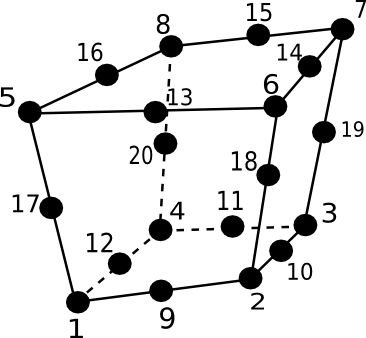
A hexa20 cell
6.2.3.4. Canonical elements
Besides Amelet HDF defines some canonical geometrical elements.
Note
the vector connecting the initial node i with the terminating node j is written \(\overrightarrow{N_{ij}}\)
- plane
- A plane is made up of 3 nodes.
- \(\overrightarrow{V_{12}}\) must not be aligned with \(\overrightarrow{V_{13}}\)
- The order of nodes gives the plane orientation, the normal is defined by \(\vec{n} = \overrightarrow{V_{12}} \times \overrightarrow{V_{13}}\)
- code : 15
- A plane is made up of 3 nodes.
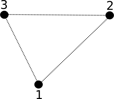
A plane element
- circle
- A circle is defined by three nodes :
- The node 1 is the center of the circle
- The node 2 gives the radius
- The node 3 gives the plane containing the circle
- \(\overrightarrow{V_{12}}\) must not be aligned with \(\overrightarrow{V_{13}}\)
- The order of nodes gives the plane orientation, the normal is defined by \(\vec{n} = \overrightarrow{V_{12}} \times \overrightarrow{V_{13}}\)
- code : 16
- A circle is defined by three nodes :
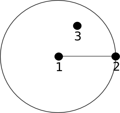
A circle element
- ellipse
- An ellipse is defined by three nodes :
- Node 1 and node 2 are the foci
- The node 3 is on the ellipse and gives the “radius” as well as the plane which contains the ellipse
- \(\overrightarrow{V_{12}}\) must not be aligned with \(\overrightarrow{V_{13}}\)
- The order of nodes gives the plane orientation, the normal is defined by \(\vec{n} = \overrightarrow{V_{12}} \times \overrightarrow{V_{13}}\)
- code : 17
- An ellipse is defined by three nodes :
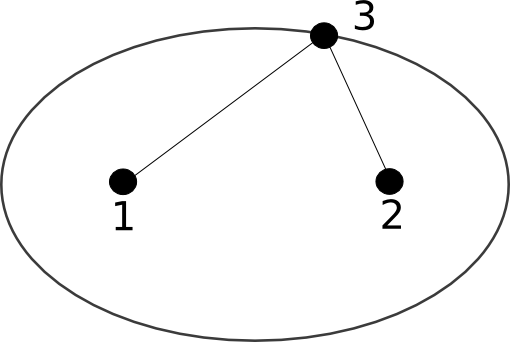
An ellipse element
- cylinder
- A cylinder is defined by three nodes :
- The node 1 is the center of the base circle
- The node 2 gives the radius of the base circle
- The node 3 is the center of the top circle.
- Nodes 1 and 3 are the axis of the cylinder.
- \(\overrightarrow{V_{12}}\) and \(\overrightarrow{V_{13}}\) are orthogonal
- code : 105
- A cylinder is defined by three nodes :
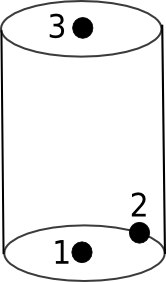
A cylinder element
- cone
- A cone is defined by four nodes :
- The node 1 is the center of the base circle
- The node 2 gives the radius of the base circle
- The node 3 is the center of the top circle
- The node 4 gives the radius of the top circle.
- Nodes 1 and 3 gives the axis of the cone.
- \(\overrightarrow{V_{13}}\) and \(\overrightarrow{V_{12}}\) are orthogonal
- \(\overrightarrow{V_{13}}\) and \(\overrightarrow{V_{34}}\) are orthogonal
- code : 106
- A cone is defined by four nodes :
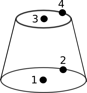
A cone element
- sphere
- A sphere is defined by two nodes :
- The node 1 is the center of the sphere
- The node 2 gives the radius of the sphere
- code : 107
- A sphere is defined by two nodes :
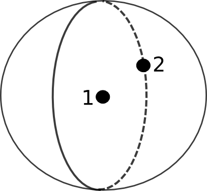
A sphere element
6.2.3.5. The elementTypes dataset
/mesh/$gmesh/$mesh/elementTypes is a one dimensional 8-bits integer dataset
and gives the type of all elements in the mesh.
Warning
/mesh/$gmesh/$mesh/elementTypes is a 8-bits integer dataset
The size of elementTypes is the number of elements.
Note
It is simple to compute the number of elements of a given type by summing
the number of time a type appears in elementTypes.
| index | Element’s types |
|---|---|
| 0 | 1 |
| 1 | 2 |
| 2 | 11 |
In this example, three elements are defined (two bar2 and one tri3). The index is implicit.
The genuine dataset is
| 1 |
| 2 |
| 102 |
6.2.3.6. Recap table
| 1D | |
| bar2 | 1 |
| bar3 | 2 |
| 2D | |
| tri3 | 11 |
| tri6 | 12 |
| quad4 | 13 |
| quad8 | 14 |
| plane | 15 |
| circle | 16 |
| ellipse | 17 |
| 3D | |
| tetra4 | 101 |
| pyra5 | 102 |
| penta6 | 103 |
| hexa8 | 104 |
| cylinder | 105 |
| cone | 106 |
| sphere | 107 |
| tetra10 | 108 |
| hexa20 | 109 |
6.2.4. elementNodes
Elements are defined by the nodes. The type of the element gives the number
of nodes, the dataset elementNodes gives the nodes involved in the
element definition.
/mesh/$gmesh/$mesh/elementNodes is a one dimensional integer dataset.
For each row of /mesh/$gmesh/$mesh/elementTypes, there is a matching
number_of_nodes.
In /mesh/$gmesh/$mesh/elementNodes there are number_of_nodes rows indicating
the index of each involved nodes (defined in /mesh/$gmesh/$mesh/nodes).
Example for the following /mesh/$gmesh/$mesh/elementTypes :
| 1 |
| 1 |
| 11 |
and /mesh/$gmesh/$mesh/elementNodes is
| index | Element’s node |
|---|---|
| 0 | 0 |
| 1 | 1 |
| 2 | 1 |
| 3 | 2 |
| 4 | 0 |
| 5 | 2 |
| 6 | 3 |
According to the preceding elementTypes example :
- The first bar2 is defined by the nodes 0 and 1
- The second bar2 by the nodes 1 and 2
- The tri3 by the nodes 0, 2 et 3.
The genuine dataset is without headers :
| 0 |
| 1 |
| 1 |
| 2 |
| 0 |
| 2 |
| 3 |
6.2.5. group
Until now, a mesh is a set of nodes and a set of elements. CAD or topology areas
(like plane’s wings, thin wires) are groups (of elements for instance). Those
groups are /mesh/$gmesh/$mesh/group‘s children.
/mesh/$gmesh/$mesh/group is an HDF5 group and contains HDF5 integer datasets.
These datasets are either sets of nodes indices from /mesh/$gmesh/$mesh/nodes
(the attribute type equals node)
or sets of elements indices from /mesh/$gmesh/$mesh/elementTypes (the attribute
type equals element).
If type equals element the group has another attribute : entityType.
entityType is an hdf5 string attribute and gives the type of entities
stored in the group. entityType can take the following values :
edge: the group contains only edge elements.face: the group contains only surface elements.volume: the group contains only volume elements.
Name’s length of datasets must have less than 20 characters.
Example :
data.h5
`-- mesh/
    `-- $gmesh1/
        `-- $plane[@type=unstructured]/
            |-- nodes
            |-- elementTypes
            |-- elementNodes
            `-- group
                |-- $field-location[@type=node]
                |-- $right-wing[@type=element
                |               @entityType=face]
                `-- $left-wing[@type=element
                               @entityType=face]
/mesh/$gmesh1/$mesh1 has three groups :
$field-location, a node group which the location where the field will be computed.$right-wing, an element group which reprensets the right wing of a plane$left-wing, an element group which reprensets the left wing of a plane
For example /mesh/$gmesh1/$mesh1/group/$field-location is
| index | indices of nodes from /mesh/$gmesh1/$mesh1/nodes |
|---|---|
| 0 | 0 |
| 1 | 1 |
| 2 | 1 |
| 3 | 2 |
| 4 | 0 |
| 5 | 2 |
| 6 | 3 |
The index and headers are reported for convenience.
6.2.6. groupGroup
groupGroup is an HDF5 group and contains sets of group children.
groupGroup children are named HDF5 datasets of 20 character
string, each groupGroup is a set group’s names.
Name’s length of sets must have less than 20 characters.
Example :
data.h5
`-- mesh/
    `-- $gmesh1/
        `-- $mesh1[@type=unstructured]/
            |-- nodes
            |-- elementTypes
            |-- elementNodes
            |-- group
            |   |-- $field-location[@type=node]
            |   |-- $right-wing[@type=element
            |   |               @entityType=face]
            |   `-- $left-wing[@type=element]
            |                  @entityType=face]
            `-- groupGroup
                `-- $wings
and /mesh/$gmesh1/$mesh1/groupGroup/$wings is
| index | /mesh/$gmesh1/$mesh1/group‘s children names |
|---|---|
| 0 | $right-wing |
| 1 | $left-wing |
The index and headers are reported for convenience.
Note
It is possible to create groupGroups of groupGroups.
6.3. Structured mesh
The main difference between an unstructured mesh and a structured mesh is that
the nodes and the elements of a structured mesh are implicitly defined by a grid.
A cartesian grid is characterized by three real vectors of
x, y and z .
Therefore elements can be located by 3 integers (i, j, k) that are the
integer coordinates in the grid.
A structured mesh is a named HDF5 group child of /mesh having an attribute
type equals structured.
A structured mesh is composed of three children :
- A mandatory child :
- a
cartesianGridgroup
- a
- Two optional children :
- a
groupHDF5 group - a
groupGroupHDF5 group
- a
Structured meshes are mainly used in electromagnetism by the Finite Difference Time Domain method (FDTD).
6.3.1. Cartesian grid
A cartesian grid is defined by 1 to 3 axis (vectors) and is the equivalent structure of the set (nodes, elementTypes, elementNodes) for an unstructured mesh. The nodes are the intersection of axis, the elementTypes is implicit because elements type is bar, face or hexa (depending on the dimension) and elementNodes are all bar, face or hexa located by their coordinates (i, j, k).
If the grid’s dimension is 1, the cartesian grid is defined by a child
vector (one dimensional dataset) called x :
data.h5
`-- mesh/
    `-- $gmesh1/
        `-- $structured-mesh-1d[@type=structured]/
            `-- cartesianGrid
                `-- x[@floatingType=vector
                      @physicalNature=length
                      @unit=meter]
x is a floatingType = vector, i.e. one dimensional dataset of reals,
its optional attributes are :
- the optional attribute
floatingType=vector - The optional attribute
physicalNaturevalue islength - The optional attribute
unitvalue ismeter
This attribute are optional because Amelet HDF specification set them.
If the grid dimension is 2, the cartesian grid is defined by 2 children floatingType called x, y :
data.h5
`-- mesh/
    `-- $gmesh1/
        `-- $structured-mesh-2d[@type=structured]/
            `-- cartesianGrid
                |-- x[@floatingType=vector
                |     @physicalNature=length
                |     @unit=meter]
                `-- y[@physicalNature=length
                      @unit=meter]
If the grid dimension is 3, the cartesian grid is defined by 3 children floatingType called x, y and z :
data.h5
`-- mesh/
    `-- $gmesh1
        `-- $structured-mesh-3d[@type=structured]/
            `-- cartesianGrid
                |-- x[@physicalNature=length
                |     @unit=meter]
                |-- y[@physicalNature=length
                |     @unit=meter]
                `-- z[@physicalNature=length
                      @unit=meter]
the physical nature of x, y and z is length and the unit is meter.
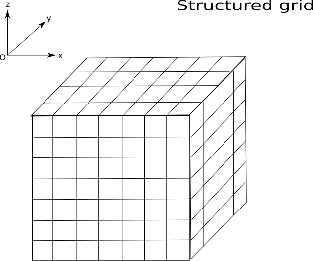
A structured orthogonal grid
6.3.1.1. Element numbering
Two manners exist to locate/describe elements and structured sets of elements.
- The numbering by indices :
Elements are located by their indices in the cartesian grid :
- i in 1D
- (i, j) in 2D
- (i, j, k) in 3D
- The implicit numbering : Elements are located by a conventional numbering rule. Every element has an integer number.
Here is an example on implicit numbering :
- for a
nx1D grid : the number of the ith element is its indexi - for a
nx * ny2D grid, the number of the (i, j) element isi+(j-1)*nx - for a
nx * ny * nz3D grid, the number of the (i, j, k)th element isi + (j-1)*nx + (k-1)*ny*nx
For a 3D grid, the index increases rapidly. A 5000x1000x1000 grid implies 5 000 000 000 mesh cells. However, the maximum 32 bit integer is 4 294 967 296 and we should use 64 bit integer to express the implicit index. The gain is not obvious relative the complexity of the convention. Therefore, the implicit numbering is not used in Amelet HDF.
Moreover, in the manner of unstructured mesh elements (see elementTypes) , Amelet HDF introduces the sub-element concept to structured mesh. With an explicit numbering, it is possible to select an element’s sub-part like a cube’s edge.
6.3.1.1.1. Node
A node is defined by an integer tuple, the size of the tuple depends on the space dimension :
| Space dimension | A’s coordinates |
|---|---|
| 1D | i |
| 2D | (i, j) |
| 3D | (i, j, k) |
Warning
The indexes of the nodes begins with 0
The nodes numbering inside a cell is defined in the same manner as :
6.3.1.1.2. Edge
An edge is defined with two aligned nodes A & B. Following the space dimension, A’s and B’s indices can take values reported in the tabular hereafter :
| Space dimension | A’s coordinates | B’s coordinates |
|---|---|---|
| 1D | i | i+1 |
| 2D | (i, j) | (i+1, j) |
| (i, j) | (i, j+1) | |
| 3D | (i, j, k) | (i+1, j, k) |
| (i, j, k) | (i, j+1, k) | |
| (i, j, k) | (i, j, k+1) |
The edges numbering inside a cell is defined in the same manner as :
6.3.1.1.3. Face
A face is defined with two nodes A & B. Following the space dimension, A’s and B’s indices can take values reported in the tabular hereafter :
| Space dimension | A’s coordinates | B’s coordinates |
|---|---|---|
| 2D | (i, j) | (i+1, j+1) |
| 3D | (i, j, k) | (i+1, j+1, k) |
| (i, j, k) | (i, j+1, k+1) | |
| (i, j, k) | (i+1, j, k+1) |
The faces numbering inside a cell is defined in the same manner as :
6.3.1.1.4. Volume
A volume is defined with two nodes A & B.
| Space dimension | A’s coordinates | B’s coordinates |
|---|---|---|
| 3D | (i, j, k) | (i+1, j+1, k+1) |
6.3.2. group
group is an HDF5 group and contains sets of nodes and sets of elements.
group children are named HDF5 dataset of integers.
Name’s length of sets must have less than 20 characters.
6.3.2.1. Nodes group
A nodes group of a structured mesh is an HDF5 two dimensional dataset children
of /mesh/$gmesh/$mesh.
A nodes group has an HDF5 attribute type, its value is node.
The first dimension is the rows. Each row defines a node by 3 integers representing the coordinates of the node.
Example :
data.h5
`-- mesh
    `-- $gmesh1
        `-- $mesh1[@type=structured]/
            |-- cartesianGrid
            `-- group
                `-- $e-field[@type=node]
where data.h5:/mesh/$gmesh1/$mesh1/group/$e-field is :
i |
j |
k |
| 1 | 1 | 1 |
| 8 | 10 | 2 |
| 15 | 15 | 15 |
Headers are reported for convenience.
6.3.2.2. Elements group
An elements group of a structured mesh is an HDF5 two dimensional dataset
children of /mesh/$gmesh/$mesh.
An elements group has an HDF5 attribute type, its value is element,
in addtition, it has the entityType attribute.
entityType is an hdf5 string attribute and gives the type of entities
stored in the group. entityType can take the following values :
edge: the group contains only edge elements.face: the group contains only surface elements.volume: the group contains only volume elements.
The first dimension is the rows. Each row defines 6 integers representing the lowest corner and the highest corner of a parallelepiped.
The lowest corner indices are the imin, jmin, kmin and
the highest corner indices are imax, jmax and kmax.
Example :
data.h5
`-- mesh/
    `-- $gmesh1/
        `-- $mesh1[@type=structured]/
            |-- cartesianGrid
            `-- group
                `-- $right-wing[@type=element
                                @entityType=volume]
where data.h5:/mesh/$gmesh1/$mesh1/group/$right-wing is :
imin |
jmin |
kmin |
imax |
jmax |
kmax |
| 1 | 1 | 1 | 12 | 10 | 12 |
| 15 | 15 | 15 | 27 | 25 | 27 |
The parallelepiped ((imin, jmin, kmin), (imax, jmax, kmax)) represents either a single element or a set of elements.
If type equals element the group has another attribute : entityType.
entityType is an hdf5 string attribute and gives the type of entities
stored in the group. entityType can take the following values :
edge: the group contains only edge elements.face: the group contains only surface elements.volume: the group contains only volume elements.
6.3.3. The normal group
The normals definition is usually related to the surface concept. However this can be also applied to the edges.
6.3.3.1. Normals of faces
In Amelet HDF
specification, normal faces are contained in the /mesh/$gmesh/$mesh/normal
group in datasets named as the initial face group in /mesh/$gmesh/$mesh/group.
The possible values of the /mesh/$gmesh/$mesh/normal/$normal dataset are :
- x+ : the normal is along the x axis and positively oriented.
- x- : the normal is along the x axis and negatively oriented.
- y+ : the normal is along the y axis and positively oriented.
- y- : the normal is along the y axis and negatively oriented.
- z+ : the normal is along the z axis and positively oriented.
- z- : the normal is along the z axis and negatively oriented.
Example :
data.h5
`-- mesh/
    `-- $gmesh1/
        `-- $mesh1[@type=structured]/
            |-- cartesianGrid
            |-- group
            |   `-- $right-wing[@type=element
            |                   @entityType=face]
            `-- normal/
                `-- $right-wing
where data.h5:/mesh/$gmesh1/$mesh1/group/$right-wing is :
imin |
jmin |
kmin |
imax |
jmax |
kmax |
| 1 | 1 | 1 | 12 | 10 | 12 |
| 15 | 15 | 15 | 27 | 25 | 27 |
and data.h5:/mesh/$gmesh1/$mesh1/normal/$right-wing is :
normal |
| x+ |
| y+ |
In the example data.h5:/mesh/$gmesh1/$mesh1/group/$right-wing are the normals
of the face group data.h5:/mesh/$gmesh1/$mesh1/normal/$right-wing.
Note
The number of rows of data.h5:/mesh/$gmesh1/$mesh1/group/$right-wing and
data.h5:/mesh/$gmesh1/$mesh1/normal/$right-wing must be equal.
6.3.3.2. Normals of edges
In Amelet HDF, structured edges are defined by six integers : imin, jmin, kmin, imax, jmax, kmax. By extension and by misnomer the normals give the direction of edges.
The same conventions as for surfaces are applied.
6.3.4. groupGroup
groupGroup is an HDF5 group and contains sets of group children.
groupGroup children are named HDF5 dataset of 20 characters
string, each groupGroup is a set group’s names.
Name’s length of sets must have less than 20 characters.
Example :
data.h5
`-- mesh/
    `-- $gmesh1
        `-- mesh1[@type=structured]/
            |-- cartesianGrid
            |-- group
            |   |-- $field-location[@type=node]
            |   |-- $right-wing[@type=element
            |   |               @entityType=cell]
            |   `-- $left-wing[@type=element
            |                  @entityType=cell]
            `-- groupGroup
                `-- $wings
and /mesh/$gmesh1/$mesh1/groupGroup/$wings is
| index | /mesh/$gmesh1/$mesh1/group‘s children names |
|---|---|
| 0 | $right-wing |
| 1 | $left-wing |
The index is implicit reported for convenience.
Note
It is possible to create groupGroups of groupGroups.
6.4. Selector on mesh
In a mesh, nodes are necessary contained in the nodes dataset.
However, it could be interesting to spot the middle of an edge or the center
of a face...
Similarly, it could nice to select a face edge without creating an edge element
in elementTypes.
This is the role of
the /mesh/$gmesh/$mesh/selectorOnMesh group localized in mesh instances :
data.h5/
`-- mesh
    `-- $gmesh1
        |-- $mesh1
        |   |-- nodes
        |   |-- elementTypes
        |   |-- elementNodes
        |   |-- group
        |   |-- groupGroup
        |   `-- selectorOnMesh
        |-- $mesh-two
        |-- $mesh-3
        |   |-- nodes
        |   |-- elementTypes
        |   |-- elementNodes
        |   |-- group
        |   |-- groupGroup
        |   `-- selectorOnMesh
        |-- $mesh#5
        |-- $mesh_6
        `-- meshLink
The selectorOnMesh group offers the mean to select and label mesh points and
mesh sub-element (The meshLink group will be covered in the next section).
selectorOnMesh is an HDF5 group which contains two kind of children :
- named tables
- named integer datasets
6.4.1. selectorOnMesh of pointInElement type
A selectorOnMesh of pointInElement type is a named table which
contains point definitions in element’s local coordinate systems. The shape of
the table depends on the unstructured | structured nature of the mesh.
The table has a string attribute named type of value pointInElement :
data.h5/
`-- mesh/
    `-- $gmesh1/
        `-- $mesh1/
            |-- nodes
            |-- elementTypes
            |-- elementNodes
            |-- group/
            |-- groupGroup/
            `-- selectorOnMesh/
                `-- $point_in_element[@type=pointInElement]
6.4.1.1. Unstructured mesh
It is possible to spot a point in an element thanks to a local coordinate system built by one, two or three vectors (depending on the dimension of the element).
Definition : \(\vec{e_{ij}}\) is the vector starting from the node i toward the node j of an element.
if E is a one-dimensional element, only \(\vec{v_1}\) is used and is defined by :
Cell \(\vec{v_1}\) bar2 \(\vec{e_{12}}\) bar3 \(\vec{e_{12}}\) In the \((O, \vec{v_1})\) coordinate system (O is node 1), the identification of a point \(P\) is realized by the vector \(\overrightarrow{OP}\) using a real number \(\alpha\) : \(\overrightarrow{OP} = \alpha \vec{v_1}\), \(P\) must be in the element.
if E is a two-dimensional element, \((\vec{v_1}, \vec{v_2})\) are used and are defined by :
Cell \(\vec{v_1}\) \(\vec{v_2}\) tri3 \(\vec{e_{12}}\) \(\vec{e_{13}}\) tri6 \(\vec{e_{12}}\) \(\vec{e_{13}}\) quad4 \(\vec{e_{12}}\) \(\vec{e_{14}}\) quad8 \(\vec{e_{12}}\) \(\vec{e_{14}}\) In the \((O, \vec{v_1}, \vec{v_2})\) coordinate system (O is node 1), the identification of a point \(P\) is realized by the vector \(\overrightarrow{OP}\) using two real numbers \(\alpha, \beta\) : \(\overrightarrow{OP} = \alpha \vec{v_1} + \beta \vec{v_2}\), \(P\) must be in the element.
if E is a three-dimension cell, \((\vec{v_1}, \vec{v_2}, \vec{v_3})\) are used and are defined by :
Cell \(\vec{v_1}\) \(\vec{v_2}\) \(\vec{v_3}\) tetra4 \(\vec{e_{12}}\) \(\vec{e_{13}}\) \(\vec{e_{14}}\) pyra5 \(\vec{e_{12}}\) \(\vec{e_{14}}\) \(\vec{e_{15}}\) penta6 \(\vec{e_{12}}\) \(\vec{e_{14}}\) \(\vec{e_{13}}\) hexa8 \(\vec{e_{12}}\) \(\vec{e_{14}}\) \(\vec{e_{15}}\) In the \((O, \vec{v_1}, \vec{v_2}, \vec{v_3})\) coordinate system (O is node 1), the identification of a point \(P\) is realized by the vector \(\overrightarrow{OP}\) using three real numbers \(\alpha, \beta, \gamma\) : \(\overrightarrow{OP} = \alpha \vec{v_1} + \beta \vec{v_2} + \gamma \vec{v_3}\), \(P\) must be in the element.
Note
The default value of a v* is -1, it is the “not used” value.
Therefore, pointInElement selectorOnMesh is a four columns HDF5 table.
| index | v1 | v2 | v3 |
The four columns are :
index: the index of the element in the list of elements (elementTypes).indexis an integer.v1: the relative distance \(\alpha\) along \(\vec{v_1}\).v1is realv2: the relative distance \(\beta\) along \(\vec{v_2}\).v2is realv3: the relative distance \(\gamma\) along \(\vec{v_3}\).v3is real
Warning
Distances are normalized
Examples for the mesh data.h5:/mesh/$gmesh1/mesh1 :
data.h5/
`-- mesh
    `-- $gmesh1
        `-- $mesh1[@type=unstructured]
            |-- nodes
            |-- elementTypes
            |-- elementNodes
            |-- group
            |   |-- $field-location[@type=node]
            |   |-- $right-wing[@type=element]
            |   `-- $left-wing[@type=element]
            |-- groupGroup
            |   `-- $wings
            `-- selectorOnMesh
                 `-- $points_in_elements[@type=pointInElement]
/mesh/$gmesh1/$mesh1/elementTypes is (implicit index are not reported),
the mesh is composed of two bar2 element.
| 1 |
| 1 |
and data.h5:/mesh/$gmesh1/$mesh1/selectorOnMesh/$points_in_elements is
| index | v1 | v2 | v3 |
| 0 | 0.5 | -1 | -1 |
| 1 | 0.5 | -1 | -1 |
This example defines the center of the two edges.
6.4.1.2. Structured mesh
selectorOnMesh of pointInElement type defines named entities referenced
relative to an element E.
A point can be localized in the element by a local coordinate system
\((\vec{v_1}, \vec{v_2}, \vec{v_3})\) (in the 3D case).
if E is an edge, \(\vec{v_1}\) is used
If E is directed along \(\overrightarrow{Ox}\),
- \(\vec{v_1} = \overrightarrow{dx}\)
If E is directed along \(\overrightarrow{Oy}\),
- \(\vec{v_1} = \overrightarrow{dy}\)
If E is directed along \(\overrightarrow{Oz}\),
- \(\vec{v_1} = \overrightarrow{dz}\)
if E is a face, \((\vec{v_1}, \vec{v_2})\) are used
- If E is in \(xOy\)
- \(\vec{v_1} = \overrightarrow{dx}\)
- \(\vec{v_2} = \overrightarrow{dy}\)
- If E is in \(xOz\)
- \(\vec{v_1} = \overrightarrow{dx}\)
- \(\vec{v_2} = \overrightarrow{dz}\)
- If E is in \(yOz\)
- \(\vec{v_1} = \overrightarrow{dy}\)
- \(\vec{v_2} = \overrightarrow{dz}\)
- If E is in \(xOy\)
if E is a volume, \((\vec{v_1}, \vec{v_2}, \vec{v_3})\) are used
- \(\vec{v_1} = \overrightarrow{dx}\)
- \(\vec{v_2} = \overrightarrow{dy}\)
- \(\vec{v_3} = \overrightarrow{dz}\)
\(\vec{dx} (respectively \vec{dy}\) and \(\vec{dz}\)) is the oriented dimension of the cell along x-axis, (respectively y-axis z-axis).
Note
The default value of a v* is -1, it is the “not used value”.
Therefore, pointInElement selectorOnMesh is a nine columns HDF5 table.
| imin | jmin | kmin | imax | jmax | kmax | v1 | v2 | v3 |
The nine columns are :
imin: the i index of the bottom corner node.iminis an integer.jmin: the j index of the bottom corner node.jminis an integer.kmin: the k index of the bottom corner node.kminis an integer.imax: the i index of the top corner node.imaxis an integer.jmax: the j index of the top corner node.jmaxis an integer.kmax: the k index of the top corner node.kmaxis an integer.v1: distance in the direction x.v1is a real.v2: distance in the direction y.v2is a real.v3: distance in the direction z.v3is a real.
Note
The following rules must be followed :
- (
imax-imin) = 0 or 1 - (
jmax-jmin) = 0 or 1 - (
kmax-kmin) = 0 or 1
One can see that if :
imin=imaxorjmin=jmaxorkmin=kmaxE is a faceimin=imaxand (jmin=jmaxorkmin=kmax) E is an edge (and respectively for the other permutations)
Examples for the mesh data.h5:/mesh/$gmesh1/$mesh1 :
data.h5/
`-- mesh/
    `-- $gmesh1/
        `-- $mesh1[@type=structured]/
            |-- cartesianGrid
            |-- group/
            |   `-- $e-field[@type=node]
            |-- groupGroup/
            `-- selectorOnMesh/
                `-- $points_in_elements[@type=pointInElement]
data.h5:/mesh/$gmesh1/$mesh1/selectorOnMesh/$points_in_elements is
| imin | jmin | kmin | imax | jmax | kmax | v1 | v2 | v3 |
|---|---|---|---|---|---|---|---|---|
| 1 | 1 | 1 | 2 | 2 | 2 | 0.5 | 0.5 | 0.5 |
| 1 | 1 | 1 | 1 | 2 | 2 | 0.5 | 0.5 | -1 |
| 1 | 1 | 1 | 1 | 1 | 2 | 0.5 | -1 | -1 |
The first point is the center of a volume, the second the center of a face and the last is the center of an edge.
6.4.2. selectorOnMesh of edge|face type
A selectorOnMesh of edge|face type is a named dataset and
defines a list of sub-elements.
The dataset has a string attribute named type of value :
edge: the dataset references edgesface: the dataset references faces
This kind of selectorOnMesh exists only for unstructured mesh since
it is natural to select whatever entity in a structured mesh thanks
the group concept.
It is possible to spot a sub-element of an element (i.e. an edge, a face)
thanks to a local numbering of sub-elements described
in Unstructured mesh. The local numbering depends on the type
attribute.
edge|face selectorOnMesh is a two columns HDF5 integer dataset.
The two columns are :
- The index of the element in the list of elements (in
elementTypes). - The number of the sub-element
Examples for the mesh data.h5:/mesh/$gmesh1/mesh1 :
data.h5/
`-- mesh
    `-- $gmesh1
        `-- $mesh1[@type=unstructured]
            |-- nodes
            |-- elementTypes
            |-- elementNodes
            |-- group
            |   |-- $field-location[@type=node]
            |   |-- $right-wing[@type=element]
            |   `-- $left-wing[@type=element]
            |-- groupGroup
            |   `-- $wings
            `-- selectorOnMesh
                 `-- $implicit_edges[@type=edge]
/mesh/$gmesh1/$mesh1/elementTypes is (implicit index are not reported).
Two bar2 and a tetra4 compose the mesh.
| 1 |
| 1 |
| 101 |
and data.h5:/mesh/$gmesh1/$mesh1/selectorOnMesh/$implicit_edges is
| 0 | 1 |
| 1 | 1 |
| 2 | 3 |
This example defines a two element edge group :
- The first edge of a bar2, it is the bar2 itself
- The third edge between node 1 and node 3 of a tetra4 cell.
6.5. The meshLink group
Sometimes a mesh can be composed of several meshes or a 2D mesh is merged with a 3D mesh. In these cases, the two meshes must be linked by defining equalities between couples of entities.
This is the task of the /mesh/$gmesh/meshLink category. A meshLink is a
named HDF5 two dimensional integer dataset with three attributes :
type, this is the type of the link defined by an HDF5 string attribute. The type can benodesorelement- If
typeisnode, the index in the dataset refer to the/mesh/$gmesh/$mesh/nodes - If
typeisedge, the index in the dataset refer to edges in/mesh/$gmesh/$mesh/elementTypes - If
typeisface, the index in the dataset refer to faces in/mesh/$gmesh/$mesh/elementTypes - If
typeisvolume, the index in the dataset refer to volumes in/mesh/$gmesh/$mesh/elementTypes
- If
mesh1, this is an HDF5 string attribute, it is the name of the first/mesh/$gmesh/$meshimplied in the link.mesh2, this is an HDF5 string attribute, it is the name of the second/mesh/$gmesh/$meshimplied in the link.
The name’s length must be less than 20 characters.
Example of /mesh/$gmesh1/meshLink :
data.h5
`-- mesh
    `-- $gmesh1
        |-- $mesh1[@type=unstructured]
        |   |-- nodes
        |   |-- elementTypes
        |   `-- elementNodes
        |-- $mesh2[@type=unstructured]
        |   |-- nodes
        |   |-- elementTypes
        |   `-- elementNodes
        |-- $mesh3[@type=structured]
        |   `-- cartesianGrid
        |-- $mesh4[@type=structured]
        |   `-- cartesianGrid
        `--meshLink
            |-- $ml1[@type=node
            |        @mesh1=/mesh/$gmesh1/$mesh1
            |        @mesh2=/mesh/$gmesh1/$mesh2]
            |-- $ml2[@type=node
            |        @mesh1=/mesh/$gmesh1/$mesh3
            |        @mesh2=/mesh/$gmesh1/$mesh4]
            |-- $ml3[@type=volume
            |        @mesh1=/mesh/$gmesh1/$mesh1
            |        @mesh2=/mesh/$gmesh1/$mesh2]
            `-- $ml4[@type=volume
                     @mesh1=/mesh/$gmesh1/$mesh3
                     @mesh2=/mesh/$gmesh1/$mesh4]
The entity in located in the selectorOnMesh/nodes table and the
selectorOnMesh/elements tables in the case of an unstructured mesh.
6.5.1. Link between two unstructured meshes
An element or node link between two unstructured meshes is defined by an HDF5 dataset with a rank of 2 and with dimensions equal number_of_entities x two. The two columns represent :
- i1 : the index i of the node in the first unstructured mesh’s
nodesdataset - i2 : the index i of the node in the second unstructured mesh’s
nodesdataset
| i1 | i2 |
|---|---|
| 0 | 0 |
| 1 | 3 |
| 2 | 6 |
Headers are reported for convenience
6.5.2. Link between two structured meshes
6.5.2.1. Nodes
A node link between two structured meshes (/mesh/$gmesh/meshLink/$ml2)
is defined by an HDF5 dataset with a rank of 2 and with dimensions equal
number_of_entities x six. The six columns represent :
- i1, j1, k1 : indices of the node in the first mesh
- i2, j2, k2 : indices of the node in the second mesh
| i1 | j1 | k1 | i2 | j2 | k2 |
|---|---|---|---|---|---|
| 1 | 1 | 1 | 2 | 2 | 2 |
| 2 | 2 | 2 | 3 | 3 | 3 |
Headers are reported for convenience
6.5.2.2. Element
An element link between two structured meshes (/mesh/$gmesh/meshLink/$ml4)
is defined by an HDF5 dataset with a rank of 2 and with dimensions equal
number_of_entities x 12. The six columns represent :
- imin1, jmin1, kmin1, imax1, jmax1, kmax1 : indices of the element in the first mesh
- imin2, jmin2, kmin2, imax2, jmax2, kmax2 : indices of the element in the second mesh
| imin1 | jmin1 | kmin1 | imax1 | jmax1 | kmax1 | imin2 | jmin2 | kmin2 | imax2 | jmax2 | kmax2 |
|---|---|---|---|---|---|---|---|---|---|---|---|
| 1 | 1 | 1 | 2 | 2 | 2 | 1 | 1 | 1 | 2 | 2 | 2 |
| 2 | 2 | 2 | 1 | 1 | 1 | 2 | 2 | 2 | 3 | 3 | 3 |
Headers are reported for convenience
6.5.3. Link between one unstructured mesh and one structured mesh
6.5.3.1. Nodes
An node link between one unstructured mesh and one structured mesh is defined by an HDF5 dataset with a rank of 2 and with dimensions equal number_of_entities x four. The four columns represent :
- i1 : the index of the node in the unstructured mesh’s
nodes - i2, j2, k2 : indices of the node in the second mesh
| i1 | i2 | j2 | k2 |
|---|---|---|---|
| 1 | 1 | 1 | 1 |
| 2 | 2 | 2 | 2 |
Headers are reported for convenience
6.5.3.2. Element
An element link between one unstructured mesh and one structured mesh is defined by an HDF5 dataset with a rank of 2 and with dimensions equal number_of_entities x seven. The seven columns represent :
- i1 : the indice of the node in the unstructured mesh’s
nodes - imin2, jmin2, kmin2, imax2, jmax2, kmax2 : indices of the element in the second mesh
| i1 | imin2 | jmin2 | kmin2 | imax2 | jmax2 | kmax2 |
|---|---|---|---|---|---|---|
| 1 | 1 | 1 | 1 | 2 | 2 | 2 |
| 2 | 2 | 2 | 2 | 3 | 3 | 3 |
Headers are reported for convenience
6.5.4. Link between one structured mesh and one unstructured mesh
6.5.4.1. Nodes
An node link between one structured mesh and one unstructured mesh is defined by an HDF5 dataset with a rank of 2 and with dimensions equal number_of_entities x four. The four columns represent :
- i1, j1, k1 : indices of the node in the second mesh
- i2 : the index of the node in the unstructured mesh’s
nodes
| i1 | j1 | k1 | i2 |
|---|---|---|---|
| 1 | 1 | 1 | 1 |
| 2 | 2 | 2 | 2 |
Headers are reported for convenience
6.5.4.2. Element
An element link between one structured mesh and one unstructured mesh is defined by an HDF5 dataset with a rank of 2 and with dimensions equal number_of_entities x seven. The seven columns represent :
- imin1, jmin1, kmin1, imax1, jmax1, kmax1 : indices of the element in the second mesh
- i2 : the index of the node in the unstructured mesh’s
nodes
| imin1 | jmin1 | kmin1 | imax1 | jmax1 | kmax1 | i2 |
|---|---|---|---|---|---|---|
| 1 | 1 | 1 | 2 | 2 | 2 | 1 |
| 2 | 2 | 2 | 3 | 3 | 3 | 2 |
Headers are reported for convenience