5. Floating type structures¶

Array data are whatever data that can be contained in a multidimensional array (also called multidimensional matrix).

An HDF5 dataset is simply a multidimensional array, the values’s type of elements in a dataset is the same for all elements. This type can be :

Integer

Real

Double

String

Complex

Besides, in physics matrices’s dimensions are often linked to physical data. For instance, the first dimension of a temporal pulse current is the time. (The time being a one dimensional array (a vector) stored in a one dimensional HDF5 dataset)

To assure this association each matrix’s dimension must be linked to a dimension dataset :

data.h5/
|-- current # One dimensional real dataset parameterized by time
`-- time    # One dimensional real dataset, current's abscissa

A second example is a current density on a surface at a given frequency, the current is a two dimensional matrix and the two dimensions are x and y that are the cartesian coordinates of a grid :

data.h5/
|-- current # Two dimensional real datasets parameterized by x and y
|-- x       # First dimension : one dimensional real dataset
`-- y       # Second dimension : One dimensional real dataset

Numeric structures of this kind (one dimensional datasets, multidimensional datasets, all manner to describing a list of numbers) are used in many cases and can be found out everywhere in an Amelet HDF file, they take the shape of HDF5 elements having an attribute named floatingType.

5.1. The `floatingType` category¶

In Amelet HDF floatingType are always children of another objects in order to give it a meaning. However, it can happen a floatingType instance is orphan, for instance the result of a simulation can be only a time, a real number. The floatingType category contains orphan floatingType.

Example (see The SingleReal type for singleReal definition) :

data.h5/
|-- floatingType/
|   `-- $flash_duration[@floatingType=singleReal
|                       @label=flash duration
|                       @physicalNature=time
|                       @unit=second
|                       @value=1e-9]
`-- simulation/
    `-- $sim1[@module=my-module
        |     @version=1.2]
        |-- inputs
        `-- outputs

with data.h5:/simulation/$sim1/outputs :

/floatingType/$flash_duration

5.2. Single types¶

Generally, Amelet HDF tries to use the simplest way to describe an element. For instance, a plane wave is defined by some attributes :

data.h5
`-- electromagneticSource
    `-- planeWave
        `-- $a-plane-wave[@xo=0.0
                          @yo=0.0
                          @zo=0.0
                          @theta=0.0
                          @phi=0.0
                          @linearPolarization=0.0]

$a-plane-wave‘s’ attributes represents real numbers, their physical nature and unit are set by Amelet HDF.

Sometimes, an attribute can be expressed by several ways. Take the electric conductivity of a material model, it could be defined with an HDF5 real attribute :

data.h5
`-- physicalModel/
    `-- volume
        `-- $water[@electricConductivity=10e-6]

However, the electric conductivity depends on the frequency, and the writing above is an approximation, the valid frequency interval is omitted.

For this case, Amelet HDF proposes a little more complex structure : the single types singleReal and singleComplex.

The electric conductivity is evenly defined with a singleReal :

data.h5
`-- physicalModel/
    `-- volume
        `-- $water
            `-- electricConductivity[@floatingType=singleReal]
                                     @value=10e-6]

5.2.1. The SingleInteger type¶

A singleInteger is a floatingType that represents a integer with optional attributes.

One mandatory attribute :

value : the value of the singleInteger, it is an HDF5 integer attribute.

Optional attributes :

label : the label of the singleInteger
physicalNature : the physical nature of the singleInteger
unit : the unit of the singleInteger
comment : a comment

These attributes are all HDF5 string attributes.

data.h5
`-- floatingType/
    `-- $an_integer[@floatingType=singleInteger
                    @value=7]

5.2.2. The SingleReal type¶

A singleReal is a floatingType that represents a real with optional attributes.

One mandatory attribute :

value : the value of the singleReal, it is an HDF5 real attribute.

Optional attributes :

label : the label of the singleReal
physicalNature : the physical nature of the singleReal
unit : the unit of the singleReal
comment : a comment

These attributes are all HDF5 string attributes.

It is usually used when an element can be defined by a single real number or an array. The electric conductivity definition of a material is a use case of the singleReal type :

data.h5
`-- physicalModel/
    `-- volume
        `-- $water
            `-- electricConductivity[@floatingType=singleReal]
                                     @value=10e-6]

5.2.3. The singleComplex type¶

A singleComplex is a floatingType that represents a complex number with optional attributes :

One mandatory attribute :

value : a two elements array (real part, imaginary part) attribute, it is the value of the complex number.

Optional attributes :

label : the label of the singleComplex
physicalNature : the physical nature of the singleComplex
unit : the unit of the singleComplex
comment : a comment

These attributes are all HDF5 string attributes.

It is usually used when an element can be defined by a single complex number or a complex array. The relative permittivity of a material is a use case of the singleComplex type :

data.h5
`-- physicalModel/
    `-- volume
        `-- $water
            `-- relativePermittivity[@floatingType=singleComplex
                                     @value=(80, 0)]

5.2.4. The singleString type¶

For the sake of completness, a singleString is a floatingType that represents a string with optional attributes :

One mandatory attribute :

value : a string attribute, it is the content of the string

Optional attributes :

label : the label of the singleComplex
physicalNature : the physical nature of the singleComplex
unit : the unit of the singleComplex
comment : a comment

These attributes are all HDF5 string attributes.

As an example, the date unit can be expressed as a singleString (see Dealing with date)

5.3. Vector¶

The next floatingType element we discuss is the vector.

A one dimensional dataset is a vector and can be explicitly defined or implicitly defined :

A vector is explicitly defined when all values are contained in the HDF5 dataset (A = [1, 2, 3, 4]), floatingType equals vector in this case
A vector is implicitly defined when its values can be computed from parameters (A = [1, 10, 2], A is the set of 5 numbers starting at 1 to 10 using a 2 spacing)

Many formulations can be used to implicitly define a vector :

linearListOfReal1 : numberOfValues evenly spaced real numbers from first to last. linearListOfReal1’s parameters are :

first : the first value of the list

last : the last value of the list

numberOfValues : the number of values in the list

linearListOfReal2 : numberOfValues evenly spaced real numbers from first using “step” spacing. linearListOfReal2’s parameters are :

first : the first value of the list

step : spacing between values

numberOfValues : the number of values in the list

logarithmListOfReal : numberOfValues evenly spaced real numbers on a logarithmic scale. logarithmListOfReal’s parameters are :

first : the first value of the list

last : the last value of the list

numberOfValues : number of values

perDecadeListOfReal : numberOfValues evenly spaced real numbers on a logarithmic scale per decade. perDecadeListOfReal’s parameters are :

first : the first value of the list

numberOfDecades : the number of decades in the list

numberOfValuesPerDecade : the number of values per decades in the list

linearListOfInteger2 : numberOfValues evenly spaced integer numbers from first using “step” spacing. linearListOfInteger2’s parameters are :

first : the first value of the list

step : spacing between values

numberOfValues : the number of values in the list

Therefore, a one dimensional HDF5 dataset with the attribute floatingType equals :

linearListOfReal1 is a linearListOfReal1 list and have also the attributes first, last and numberOfValues. The dataset’s content is not taken into account.
linearListOfReal2 is a linearListOfReal2 list and have also the attributes first, step and numberOfValues. The dataset’s content is not taken into account.
logarithmListOfReal is a logarithmListOfReal list and have also the attributes first, last and numberOfValues. The dataset’s content is not taken into account.
perDecadeListOfReal is a perDecadeListOfReal list and have also the attributes first, numberOfDecades and numberOfValuesPerDecade. The dataset’s content is not taken into account.
linearListOfInteger2 is a linearListOfInteger2 list and have also the attributes first, last and numberOfValues. The dataset’s content is not taken into account.

For example with the preceding current density data :

data.h5/
|-- $current
|-- $x[@floatingType=vector]
|-- $y[@floatingType=linearListOfReal1,
|      @first=1.0,
|      @last=10.0,
|      @numberOfValues=10]
`-- $z

$z is defined without attribute, when there is no attribute floatingType, the element is a vector.

5.3.1. Interval¶

A real interval is classically defined by two real numbers (start, end) and is written [start, end]. In Amelet HDF, a real interval is described with a linearListOfReal1 with no numberOfValues attribute.

Example :

data.h5/
`-- $int1[@floatingType=linearListOfReal1
          @physicalNature=time
          @first=0
          @last=1e-6]

data.h5:/$int1 is a time interval starting from 0 second and terminating at 1e-6 second.

5.4. Rational functions¶

5.4.1. Introduction¶

A rational function is any function which can be written as the ratio of two polynomial functions. (http://en.wikipedia.org/wiki/Rational_function).

5.4.2. The rational function¶

In Amelet HDF, rationalFunction is a floatingType, it can be found out every where in an instance. A rationalFraction is the sum of fractions of different types, the types are :

Type 1 : $f(p) = B$
Type 2 : $f(p) = \dfrac{B}{p-A}$
Type 3 : $f(p) = \dfrac{B}{(p-A)^2}$
Type 4 : $f(p) = \dfrac{B}{(p-A)^2+(2\pi F)^2}$
Type 5 : $f(p) = \dfrac{B(p-A)}{(p-A)^2+(2\pi F)^2}$

A rationalFunction is an named HDF5 table that has four columns : type, A, B and F. type is an HDF5 integer and the others are HDF5 reals.

Type 1 : only B is read
Types 2 and 3 : A and B are used
Types 4 and 5 : A, B and F are used

Example :

type	A	B	F
1		1
2	2	3
3	4	5
4	6	7	8
5	9	10	11

5.4.3. The general rational function¶

The general rational function is sometimes used to generalize the representation of frequency dependent properties of dielectric material for instance.

Two types of general rational function exist:

Polynomial
Partial fraction.

A general rational function $f(j\omega)$ of polynomial type is written as :

\[f(j\omega) = \dfrac {a_0 + a_1(j\omega) + a_2(j\omega)^2 + ... + a_n(j\omega)^n} {b_0 + b_1(j\omega) + b_2(j\omega)^2 + ... + b_n(j\omega)^n}\]

where $a_i, b_i$ are complex numbers.

A general rational function $f(j\omega)$ of partial fraction type is written as :

\[f(j\omega) = \sum_i { ( { \dfrac{a_0}{b_0} + \dfrac {a_{1}} {j\omega - b_1} + \dfrac {a_{2}} {(j\omega - b_2)^2} + ... + \dfrac {a_{i}} {(j\omega - b_i)^{k_i}} } ) }\]

where $a_i, b_i$ are complex numbers and $k_i$ are integer numbers.

In Amelet HDF, generalRationalFunction is a floatingType, it can be found out every where in an instance.

A floatingType generalRationalFunction has one more attribute:

type : type is a HDF5 character attribute which gives the type of the floatingType. It can take the values polynomial and partialFraction

5.4.3.1. General rational function of polynomial type¶

A generalRationalFunction of polynomial type is a 2 column dataset of complex numbers ( {r, i} ).

The number of lines is the degree of the rational function, example :

degree	numerator	denominator
0	(1, 2)	(2, 4)
1	(1, 1)	(0, 2)
2	(0, 2)	(2, 0)
.	.	.
.	.	.
.	.	.
n	(32, 2)	(2, -12)

The headers and the first column are represented for the explanation, the genuine dataset is :

(1, 2)	(2, 4)
(1, 1)	(0, 2)
(0, 2)	(2, 0)
.	.
.	.
.	.
(32, 2)	(2, -12)

This example defines a nth order general rational function and is equivalent to the following relation :

\[f(j\omega) = \dfrac {(1+2j) + (1+1j)(j\omega) + ( 2j)(j\omega)^2 + ... + (32+2j)(j\omega)^n} {(2+4j) + ( 2j)(j\omega) + (2 )(j\omega)^2 + ... + (2-12j)(j\omega)^n}\]

5.4.3.2. General rational function of partial fraction type¶

A generalRationalFunction of partial fraction type is an named HDF5 table that has three columns : degree of the denominator, numerator and denominator. degree is an HDF5 integer and the others are HDF5 complex numbers ( {r, i} ).

Example :

degree	numerator	denominator
0	(5, 0)	(1, 0)
1	(3, 4)	(1, 4)
2	(2, 1)	(1, 4)
1	(0, 2)	(2, 0)

This example is equivalent to this rational fraction:

\[f(j\omega) = 5 + \dfrac {3 + 4j} {j\omega - 1 - 4j} + \dfrac {2 + 1j} {(j\omega - 1 - 4j)^2} + \dfrac {2j} {j\omega - 2}\]

5.4.4. The rational¶

In order to be consistent with the floatingType dataSet relative to singleReal and singleComplex, rationalFunction can be used as element of a matrix named data. The element of data are HDF5 string, names of the rationalFunction. The resulting structure is a floatingType named rational, it is a named HDF5 group and is made up of :

An HDF5 group named function that contains rationalFunction
A dataSet named data of HDF5 string

The floatingType rational is used for the definition of impedance : (the whole definition of a /physicalModel/multiport will be seen later)

data.h5
    /physicalModel/
    `-- multiport/
        `-- $impedance1[@floatingType=rational
            |           @physicalNature=impedance]
            |-- function
            |   |-- $rationalFraction1[@floatingType=rationalFunction]
            |   |-- $rationalFraction2[@floatingType=rationalFunction]
            |   `-- $rationalFraction3[@floatingType=generalRationalFunction
            |                          @type=polynomial]
            `-- data

with /physicalModel/multiport/$impedance1/function/$rationalFraction1 :

type	A	B	F
1		1
2	2	3
3	4	5
4	6	7	8
5	9	10	11

and /physicalModel/multiport/$impedance1/function/$rationalFraction3 :

(1, 2)	(2, 4)
(1, 1)	(0, 2)
(0, 2)	(2, 0)
.	.
.	.
.	.
(32, 2)	(2, -12)

and /physicalModel/multiport/$impedance1/data :

$rationalFraction1	$rationalFraction3
$rationalFraction2	$rationalFraction1

5.5. DataSet¶

The dataSet structure is another floatingType in the Amelet HDF specification, it represents a matrix with physical quantity attributes.

A dataSet can be used to define a multiport resistance with constant values for instance :

data.h5
`-- physicalModel/
    `-- multiport/
        `-- $resistance0[@floatingType=dataSet
                         @physicalNature=resistance
                         @unit=ohm]

In the example $resistance0 is a three ports multiport (given by the dimension of HDF5 dataset), /physicalModel/multiport/$resistance0 is :

12	13	14
13	12	13
14	13	12

HDF5 provides the API to query the dimension of the dataset.

Note

DataSet is a native HDF5 object.

5.6. ArraySet¶

An arraySet is another floatingType structure, it has an attribute floatingType equals arraySet. The reason of this floating characteristic is that an arraySet is a structure that can be also used in many locations in a Amelet HDF instance.

An arraySet is defined by :

data, an HDF5 multidimensionnal dataset, its type can be :
- integer
- real
- double
- complex
- string
a “ds” group (dimension scale) that contains the HDF5 dataset representing data dimensions. If data’s dimension is 3, ds’s children are:
- dim1, first data‘s dimension. dim1 is a one dimensional dataset.
- dim2, second data‘s dimension. dim2 is a one dimensional dataset.
- dim3, third data‘s dimension. dim3 is a one dimensional dataset.
The names dim1 ... dimN is a Amelet HDF convention and are the only authorized names.

The first dimension is the most internal loop of data.

Example :

data.h5/
`-- floatingType/
    `-- $eField[@floatingType=arraySet]
        |-- data              # a (n x m x l) dataset
        `-- ds/
            |-- dim1
            |-- dim2
            `-- dim3

In addition, Amelet HDF defines the manner to write scientific data the way there is no place for misunderstanding. That’s why the physical nature and unit of parameters are set by Amelet HDF to limit the complexity of the understanding and the treatment. There is no need the write code to convert the unknown input unit toward another unit.

However, arraySets can be read out of the context of Amelet HDF, simulation results can be stored in an arraySet file and there is no way to know the function, the nature and the unit of the data.

As a consequence the arraySet structure must be self-describing and could provide optional attributes to precise the arraySet. The optional attribute hold by data (as data is a floatingType=dataSet are :

the label ( HDF5 string attribute label )
the physical nature : “length”, “voltage” ( HDF5 string attribute physicalNature )
the unit : “meter”, “volt” ( HDF5 string attribute unit )
a comment ( HDF5 string attribute comment )

In addition, the type (or the class) of the values (integer, float...) is not published by an attribute, HDF5 provide the function H5LTget_dataset_info, the returned type_class is the class of the values.

5.6.1. The dimensions order¶

The “ds” group contains the HDF5 datasets representing data dimensions : the ds/dim*. They contain as well the physical nature of the dimensions, they follow the rule :

ds/dim1 is always the fastest-changing dimension.

5.6.2. C versus fortran - Storage conventions¶

C and fortran don’t use the same storage convention :

C : the last listed dimension is the fastest-changing dimension and the first-listed dimension is the slowest changing
Fortran : Fortran stores data by columns, the first-listed dimension is the fastest-changing dimension and the last-listed dimension is the slowest-changing

As a consequence, the array A(20, 100) allocated in C is the array A(100, 20) in fortran. HDF5 uses C storage conventions so an array stored from a C program must be read in the reversed order from a fortran program, the HDF5 wrapper accomplishes the task transparently for the user.

5.6.3. Component parameter¶

Numerical data can be scalar but can also be vector fields. In this case, a dimension handle the component loop, for this dimension the @physicalNature equals component and values stored in the dataset are HDF5 string which are the label of each component.

The possible components by coordinate system are :

Coordinate system	Possible components
Cartesian coordinate system	x, y, z
Cylindrical coordinate system	r, theta, z
Spherical coordinate system	r, theta, phi

5.6.3.1. Example 1¶

Example of the components Ex, Ey, Ez of an electric field during the time

data.h5/
`-- floatingType/
    `-- $dataOne[@floatingType=arraySet
        |        @label=Electric field around a wire]
        |-- data[@label=electric field
        |        @physicalNature=electricField
        |        @unit=voltPerMeter]
        `-- ds/
            |-- dim1[@label=component x y z
            |        @physicalNature=component]
            `-- dim2[@label=the time
                     @physicalNature=time
                     @unit=second]

with data.h5:/floatingType/dataOne/ds/dim1 vector :

index	component
0	x
1	y
2	z

5.6.3.2. Example 2¶

Example of the components Ex, Ey of an electric field during the time

data.h5/
`-- floatingType/
    `-- $dataOne[@floatingType=arraySet
        |        @label=Electric field around a wire]
        |-- data[@label=electric field
        |        @physicalNature=electricField
        |        @unit=voltPerMeter]
        `-- ds/
            |-- dim1[@label=component x y
            |        @physicalNature=component]
            `-- dim2[@label=the time
                     @physicalNature=time
                     @unit=second]

with data.h5:/floatingType/dataOne/ds/dim1 vector :

index	component
0	x
1	y

5.6.4. Numerical data on mesh¶

Computations data are often located in space and a mesh is used the associate a data value to a mesh entity. In Amelet HDF this association is handled by a dim* child of the arraySet. The physicalNature of this dimension must be meshEntity.

For a complete description of mesh see Mesh.

In this case, the dim* dataset is a string dataset and the values are the name of the mesh entity.

data.h5/
|-- mesh/
|   `-- $gmesh1/
|       `-- $mesh1/
|           `-- group/
|               `-- $exchange_surface[@entityType=node]
`-- floatingType
    `-- $dataOne[@floatingType=arraySet
        |        @label=Electric field around the wire]
        |-- data[@label=electric field
        |        @physicalNature=electricField
        |        @unit=voltPerMeter]
        `-- ds/
            |-- dim1[@label=component x y z
            |        @physicalNature=component]
            |-- dim2[@label=mesh elements
            |        @physicalNature=meshEntity]
            `-- dim3[@label=the time
                     @physicalNature=time
                     @unit=second]

with /floatingType/$dataOne/ds/dim2 :

/mesh/$gmesh1/$mesh1/group/$exchange_surface

5.6.4.1. Numerical data on nodes¶

The preceding example deals with numerical data on nodes (the entityType is node), that is to say all data are located on nodes in the node group.

Considering the meshEntity dimension, from the first value to last value, values are located from the first node to the last node defined in the group node.

5.6.4.2. Numerical data on unstructured elements - the `location` attribute¶

Data may also be located on the elements of a mesh. The following example associates data on the barycenter of /mesh/$gmesh1/mesh1/group/$exchange_surface elements :

data.h5/
|-- mesh/
|   `-- $gmesh1/
|       `-- $mesh1/
|           `-- group/
|               `-- $exchange_surface[@entityType=face]
`-- floatingType/
    `-- $dataOne[@floatingType=arraySet
        |        @label=Electric field around the wire]
        |-- data[@label=electric field
        |        @physicalNature=electricField
        |        @unit=voltPerMeter]
        `-- ds/
            |-- dim1[@label=component x y z
            |        @physicalNature=component]
            |-- dim2[@label=mesh elements
            |        @physicalNature=meshEntity]
            `-- dim3[@label=the time
                     @physicalNature=time
                     @unit=second]

with /floatingType/$dataOne/ds/dim2 :

/mesh/$gmesh1/mesh1/group/$exchange_surface

The example deals with numerical data on elements (the entityType is face), that is to say all data are located on elements in the group.

But how are data located within the element ? The answer is in the location attribute.

When physicalNature is meshEntity, the dimension can have an optional attribute named location. The location attribute is a string attribute which can take the following values :

barycenter, data are located at the barycenter of the elements.
node, data are located at element nodes.
middleEdge, data are located at element middle edges if entityType=face or entityType=volume
centerFace, data are located at element center face if entityType=volume.

If location is not present or not understood, its value is barycenter.

For this to be possible, implicit and explicit element definition are necessary :

Unstructured elements are explicitly defined by nodes. So element nodes are explicitly selectable.
In addition elementTypes details the definition of (implicit) subelements (edges for entityType=face, edges and faces for entityType=volume) of an element, these subelements are numbered.

Implicit subelements permit to select (n-1) dimensional subelements of an n dimensional element.

Important

A simple rule has to be followed to localize data on the mesh :

Data are always located on an explicit or implicit points list.

Data size must be the same as the points list size.

Data are distributed on points in the same order they are defined. If a point is already associated with a value, the process goes on with the next possible location.

5.6.4.2.1. Example 1¶

The first example deals with three reals located on triangles barycenter (one barycenter per element so three elements), the Amelet HDF structure looks like the following :

data.h5/
|-- mesh/
|   `-- $gmesh1/
|       `-- $mesh1[@type=unstructured]/
|           |-- nodes
|           |-- elementTypes
|           |-- elementNodes
|           `-- group/
|               `-- $three_triangles[@type=element
|                                    @entityType=face]
`-- floatingType/
    `-- $dataOne[@floatingType=arraySet
        |        @label=Electric field on a triangle]
        |-- data[@label=electric field
        |        @physicalNature=electricField
        |        @unit=voltPerMeter]
        `-- ds/
            `-- dim1[@label=mesh elements
                     @physicalNature=meshEntity
                     @location=barycenter]

data.h5:/mesh/$gmesh1/$mesh1/group/$three_triangles is :

14

23

5

data.h5:/floatingType/$dataOne/data is a one-dimensional real array, its length is three and data.h5:/floatingType/$dataOne/ds/dim1 is :

/mesh/$gmesh1/mesh1/group/$three_triangle

Associations between triangles and data are :

triangle 0 in ``$three_triangles`` (14) holds /floatingType/$dataOne/data[0]
triangle 1 in ``$three_triangles`` (23) holds /floatingType/$dataOne/data[1]
triangle 2 in ``$three_triangles`` (5) holds /floatingType/$dataOne/data[2]

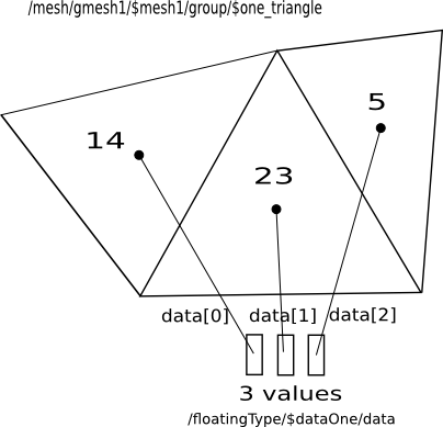
_images/data_on_element_mesh_triangles.png

Data dispatching on a triangle (tri3)

5.6.4.2.2. Example 2¶

The second example deals with six reals located on two joint quad4 nodes, the Amelet HDF structure looks like the following :

data.h5/
|-- mesh/
|   `-- $gmesh1/
|       `-- $mesh1[@type=unstructured]/
|           |-- nodes
|           |-- elementTypes
|           |-- elementNodes
|           `-- group/
|               `-- $two_quad4[@type=element
|                              @entityType=face]
`-- floatingType
    `-- $dataOne[@floatingType=arraySet
        |        @label=Electric field on a quad4]
        |-- data[@label=electric field
        |        @physicalNature=electricField
        |        @unit=voltPerMeter]
        `-- ds/
            `-- dim1[@label=mesh elements
                     @physicalNature=meshEntity
                     @location=node]

data.h5:/mesh/$gmesh1/$mesh1/group/$two_quad4 is :

12

27

data.h5:/mesh/$gmesh1/$mesh1/elementTypes is respectively for the 12th and 27th element :

...
1
2
5
6
...
2
3
4
5
...

data.h5:/floatingType/$dataOne/data is a one-dimensional real array, its length is six and data.h5:/floatingType/$dataOne/ds/dim1 is :

/mesh/$gmesh1/mesh1/group/$two_quad4

Associations between quad4 and data are :

quad4 0 in ``$two_quads4`` (12)
  node 1 holds /floatingType/$dataOne/data[0]
  node 2 holds /floatingType/$dataOne/data[1]
  node 3 holds /floatingType/$dataOne/data[2]
  node 4 holds /floatingType/$dataOne/data[3]
quad4 1 in ``$two_quads4`` (27)
  node 2 holds /floatingType/$dataOne/data[4]
  node 3 holds /floatingType/$dataOne/data[5]

Here, the first value in data is located on the first node of the first quad4, the second value on the second node, the third value on the third node of the first quad4, the fourth value on the fourth node. The other values are located on the second quad4 nodes. If the first node of the second quad4 is already associated with a value, we continue. Finally the last value is located on the only node (and last) that has no value of the second quad4.

Note

On the figure, external numbers are quad4 nodes indices defined in data.h5:/mesh/$gmesh1/$mesh1/elementTypes and data.h5:/mesh/$gmesh1/$mesh1/elementNodes and internal numbers are nodes numbers relative to the element definition see elementTypes)

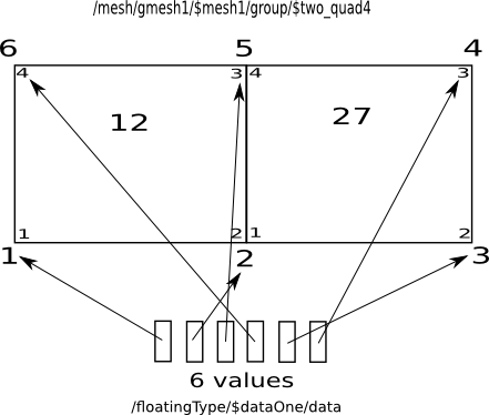
Data dispatching on quad4 nodes

This rule is valid for edges and faces.

5.6.4.3. Data and finite difference method - the `location` attribute¶

For finite difference (FD) methods under cartesian coordinate system, computed quantities are not all calculated at the same location :

Electric fields are located at cell’s middle edges
Magnetic fields are located at cell’s center faces

For instance, in a 2D Yee scheme Ex, Ey and Hx components are located as the following picture shows :

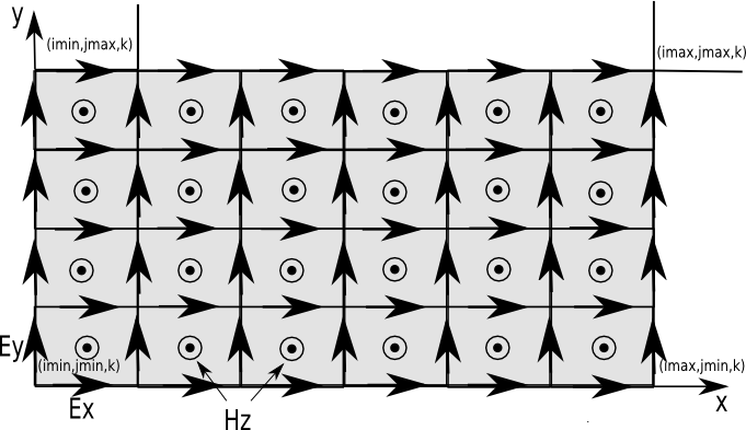
Ex, Ey and Hx location in a 2d Yee grid

In addition structured entities (volumes, surfaces and edges) are defined by too end-corner points (see the gray zone on the picture) :

(imin, jmin, kmin) are the coordinates of the inferior end-corner point
(imax, jmax, kmax) are the coordinates of the superior end-corner point

The components contained in a such entity are (the fortran notation for integer range is used, Ex(1:2) is a two elements array with Ex(1) and Ex(2)):

Ex(imin:imax-1, jmin:jmax , kmin:kmax )
Ey(imin:imax , jmin:jmax-1, kmin:kmax )
Ez(imin:imax , jmin:jmax , kmin:kmax-1)

and

Hx(imin:imax , jmin:jmax-1, kmin:kmax-1)
Hy(imin:imax-1, jmin:jmax , kmin:kmax-1)
Hz(imin:imax-1, jmin:jmax-1, kmin:kmax )

To store Ex, Ey and Ez in a single arraySet and Hx, Hy and Hz in another arraySet, a meshEntity dimension is defined by x, y, z and the shape of the regular data dataset of the arraySet is [imin:imax, jmin:jmax, kmin:kmax], as a consequence some components are written but should not be consumed :

Ex(imax, jmin:jmax , kmin:kmax )
Ey(imin:imax , jmax, kmin:kmax )
Ez(imin:imax , jmin:jmax , kmax)

and

Hx(imin:imax , jmax, kmin:kmax-1) and Hx(imin:imax , jmin:jmax-1, kmax)
Hy(imax, jmin:jmax , kmin:kmax-1) and Hy(imin:imax-1, jmin:jmax , kmax)
Hz(imax, jmin:jmax-1, kmin:kmax ) and Hz(imin:imax-1, jmax, kmin:kmax )

The location attribute

In the case of finite difference methods, the location attribute is finiteDifference

Note

Data are written in the same order the coordinate system dimension are defined. (x, y, z, or i, j, k for a cartesian coordinate system)

5.6.4.3.1. Example¶

For the the components from the image, the fields are stored as follows :

data.h5/
|-- mesh/
|   `-- $gmesh1/
|       `-- $mesh1[@type=structured]/
|           |-- cartesianGrid/
|           `-- group/
|               `-- $gray_surface[@type=element
|                                 @entityType=face]
`-- floatingType/
    `-- $ex_and_ey[@floatingType=arraySet
        |          @label=Electric field on the gray surface]
        |-- data[@label=electric field
        |        @physicalNature=electricField
        |        @unit=voltPerMeter]
        `-- ds/
           |-- dim1[@label=Ex and Ey
           |        @physicalNature=component]
           `-- dim2[@label=the grey surface
                    @physicalNature=meshEntity
                    @location=finiteDifference]

with data.h5:/floatingType/$ex_and_ey/ds/dim1 :

index	component
0	x
1	y

and data.h5:/mesh/$gmesh1/$mesh1/group/$gray_surface is :

imin

jmin

k

imax

jmax

k

5.6.5. Examples of arraySets¶

The material relative permittivity definition (in /physicalModel/volume):
- data is a one dimensional complex dataset without unit;
- ds/dim1 is a one dimensional real dataset (a vector)
  - physicalNature = “frequency”
  - unit = “hertz”
A current pulse in the time domain
- data is a one dimensional real dataset
  - physicalNature = “current”
  - Unit = “ampere”
- ds/dim1 is a one dimensional real dataset
  - physicalNature = “time”
  - unit = “second”
An electromagnetic pulse ExEy in the time domain :
- data is a two dimensional real dataset
  - physicalNature = “electricField”
  - unit attribute = “voltPerMeter”
- ds/dim1 is a one dimensional string dataset
  - physicalNature = “component”
  - unit = “”
  - values of ds/dim1 are [“x”, “y”]
- ds/dim2 is a one dimensional real dataset
  - physicalNature = “time”
  - unit = “second”
The definition of a resistance found out in the /physicalModel/resistance category :
- data is a one dimensional real dataset
  - physicalNature = “resistance”
  - unit = “ohm”
- ds/dim1 is a one dimensional real dataset
  - PhysicalNature = “frequency”
  - Unit = “hertz”

5.6.6. The `complement` group¶

An arraySet can have an optional complement group. If present, this group contains floatingType elements aiming at completing the meaning of the arraySet.

Example :

data.h5/
`-- floatingType/
    `-- $dataOne[@floatingType=arraySet
        |        @label=Current on the wire]
        |-- complement/
        |   `-- temperature[@floatingType=singleReal
        |                   @label=temperature
        |                   @physicalNature=temperature
        |                   @unit=kelvin
        |                   @value=215]
        |-- data[@label=current
        |        @physicalNature=current
        |        @unit=ampere]
        `-- ds/
            |-- dim1[@label=height
            |        @physicalNature=length
            |        @unit=meter]
            |-- dim2
            |-- dim3
            `-- dim4

In this example, data.h5:/floatingType/$dataOne is completed by the singleReal temperature.

5.6.7. ArraySet and Coordinate systems¶

For simple use cases, Amelet HDF defines conventions to express data in coordinate systems instead of creating a mesh and locating data on this mesh’s entities with the (component, entity) paradigm.

Note

Images of this section come from Wikipedia (http://www.wikipedia.org)

The convention is based upon the coordinateSystem attribute, it can take the following values :

x
xy
xyz
rtheta
rhophiz
rthetaphi

Those values are explained hereafter.

5.6.7.1. Cartesian coordinate system¶

Given the definition of the cartesian coodinate systems in 2 and 3 dimensions :

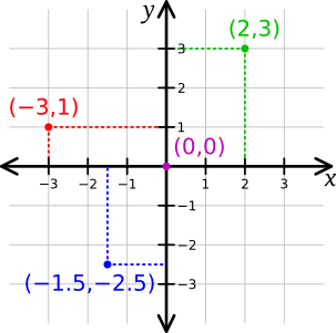
A 2D cartesian coordinate system

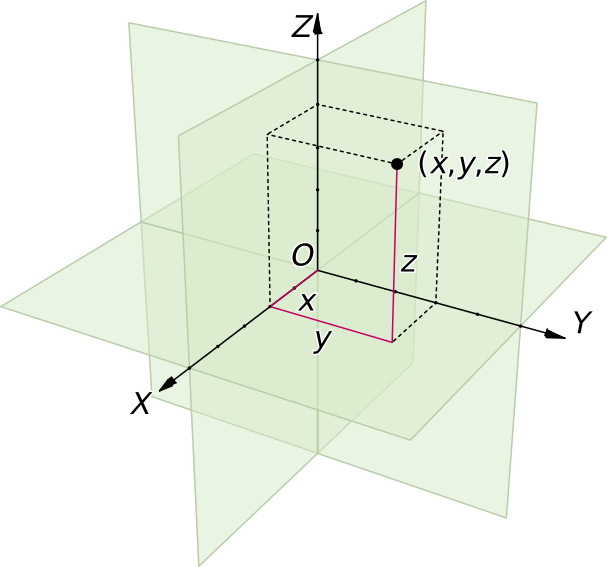
A 3D cartesian coordinate system

If an arraySet has the coordinateSystem attribute equals to x, the arraySet must have a dimension with @label equals x. This dimension represents the X axis of a one-dimensional cartesian coordinate system.
If an arraySet has the coordinateSystem attribute equals to xy, the arraySet must have two consecutive dimensions with @label equals x and @label equals y. These dimensions represent the X axis and the Y axis of a two-dimensional cartesian coordinate system.
If an arraySet has the coordinateSystem attribute equals to xyz, the arraySet must have three consecutive dimensions with @label equals x, @label equals y and @label equals z. These dimensions represent the X axis, the Y axis and the Z axis of a three-dimensional cartesian coordinate system.

Example with a three-dimensional coordinate system :

data.h5/
`-- floatingType/
    `-- $e_field[@floatingType=arraySet
        |        @coordinateSystem=xyz
        |        @label=electric field magniture in a box]
        |-- data[@label=electric field magniture
        |        @physicalNature=electricField
        |        @unit=voltPerMeter]
        `-- ds/
            |-- dim1[@label=x
            |        @physicalNature=length
            |        @unit=meter]
            |-- dim2[@label=y
            |        @physicalNature=length
            |        @unit=meter]
            `-- dim3[@label=z
                     @physicalNature=length
                     @unit=meter]

5.6.7.2. Cylindrical and polar coordinate systems¶

Given the definition of the polar coordinate system :

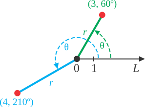
A polar coordinate system

If an arraySet has the coordinateSystem attribute equals to rtheta, the arraySet must have two consecutive dimensions with @label equals r and @label equals theta. These dimensions represent the r parameter and the theta parameter of the polar coordinate system.

Example :

data.h5/
`-- floatingType/
    `-- $e_field[@floatingType=arraySet
        |        @coordinateSystem=rtheta
        |        @label=electric field magniture in a circle]
        |-- data[@label=electric field magniture
        |        @physicalNature=electricField
        |        @unit=voltPerMeter]
        `-- ds/
            |-- dim1[@label=r
            |        @physicalNature=length
            |        @unit=meter]
            `-- dim2[@label=theta
                     @physicalNature=angle
                     @unit=degree]

Given the definition of the cylindrical coordinate system :

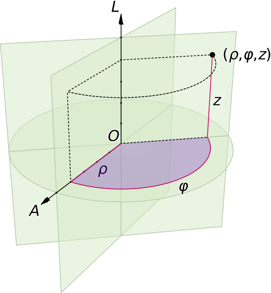
A cylindrical coordinate system

If an arraySet has the coordinateSystem attribute equals to rhophiz, the arraySet must have three consecutive dimensions with @label equals rho, @label equals phi and @label equals z. These dimensions represent the rho parameter, the phi parameter and the z parameter of the cylindrical coordinate system.

Example :

data.h5/
`-- floatingType/
    `-- $e_field[@floatingType=arraySet
        |        @coordinateSystem=rhophiz
        |        @label=electric field magniture in a cylinder]
        |-- data[@label=electric field magniture
        |        @physicalNature=electricField
        |        @unit=voltPerMeter]
        `-- ds/
            |-- dim1[@label=rho
            |        @physicalNature=length
            |        @unit=meter]
            |-- dim2[@label=phi
            |        @physicalNature=length
            |        @unit=meter]
            `-- dim3[@label=z
                     @physicalNature=angle
                     @unit=degree]

5.6.7.3. Spherical coordinate system¶

Given the definition of the spherical coordinate system :

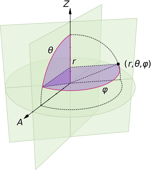
A spherical coordinate system

If an arraySet has the coordinateSystem attribute equals to rthetaphi, the arraySet must have three consecutive dimensions with @label equals r, @label equals theta and @label equals phi. These dimensions represent the r parameter, the theta parameter and the phi parameter of the spherical coordinate system.

Example :

data.h5/
`-- floatingType/
    `-- $e_field[@floatingType=arraySet
        |        @coordinateSystem=rthetaphi
        |        @label=electric field magniture in a sphere]
        |-- data[@label=electric field magniture
        |        @physicalNature=electricField
        |        @unit=voltPerMeter]
        `-- ds/
            |-- dim1[@label=r
            |        @physicalNature=length
            |        @unit=meter]
            |-- dim2[@label=theta
            |        @physicalNature=angle
            |        @unit=degree]
            `-- dim3[@label=phi
                     @physicalNature=angle
                     @unit=degree]

5.7. Expression¶

5.7.1. Overview¶

Expression is a floatingType structure which defines data by a mathematical expression thanks to embedded floatingTypes.

A floatingType expression is an HDF5 group with a mandatory HDF5 string attribute named expression, it gives the value of the expression.

As usual, common floatingType attributes (label, comment, physicalNature and unit) are optional.

Example :

data.h5
|
`-- floatingType/
    `-- $U[@floatingType=expression
        |  @expression=$R*$I
        |  @physicalNature=voltage
        |  @unit=volt]
        |-- $R[@floatingType=dataSet
        |      @physicalNature=impedance
        |      @unit=ohm]
        `-- $I[@floatingType=dataSet
               @physicalNature=current
               @unit=ampere]

In the example $U is defined by the multiplication of $R and $I.

5.7.2. Simple cases¶

In the case of common binary operators +, -, *, /, Amelet HDF defines the following shortcut :

The expression is reduced to the operator sign
Operands are named operand1 and operand2

Example : the preceding floatingType data.h5:/floatingType/$U can be re-written as :

data.h5
|
`-- floatingType/
    `-- $U[@floatingType=expression
        |  @expression=*
        |  @physicalNature=voltage
        |  @unit=volt]
        |-- operand1[@floatingType=dataSet
        |            @physicalNature=impedance
        |            @unit=ohm]
        `-- operand2[@floatingType=dataSet
                     @physicalNature=current
                     @unit=ampere]

5. Floating type structures¶

5.1. The floatingType category¶

5.2. Single types¶

5.2.1. The SingleInteger type¶

5.2.2. The SingleReal type¶

5.2.3. The singleComplex type¶

5.2.4. The singleString type¶

5.3. Vector¶

5.3.1. Interval¶

5.4. Rational functions¶

5.4.1. Introduction¶

5.4.2. The rational function¶

5.4.3. The general rational function¶

5.4.3.1. General rational function of polynomial type¶

5.4.3.2. General rational function of partial fraction type¶

5.4.4. The rational¶

5.5. DataSet¶

5.6. ArraySet¶

5.6.1. The dimensions order¶

5.6.2. C versus fortran - Storage conventions¶

5.6.3. Component parameter¶

5.6.3.1. Example 1¶

5.6.3.2. Example 2¶

5.6.4. Numerical data on mesh¶

5.6.4.1. Numerical data on nodes¶

5.6.4.2. Numerical data on unstructured elements - the location attribute¶

5.6.4.2.1. Example 1¶

5.6.4.2.2. Example 2¶

5.6.4.3. Data and finite difference method - the location attribute¶

5.6.4.3.1. Example¶

5.6.5. Examples of arraySets¶

5.6.6. The complement group¶

5.6.7. ArraySet and Coordinate systems¶

5.6.7.1. Cartesian coordinate system¶

5.6.7.2. Cylindrical and polar coordinate systems¶

5.6.7.3. Spherical coordinate system¶

5.7. Expression¶

5.7.1. Overview¶

5.7.2. Simple cases¶

5.1. The `floatingType` category¶

5.6.4.2. Numerical data on unstructured elements - the `location` attribute¶

5.6.4.3. Data and finite difference method - the `location` attribute¶

5.6.6. The `complement` group¶